Advanced Learning Algorithms

Neural networks intuition

Origins: Algorithms that try to mimic the brain

Tip

Demand Prediction Example

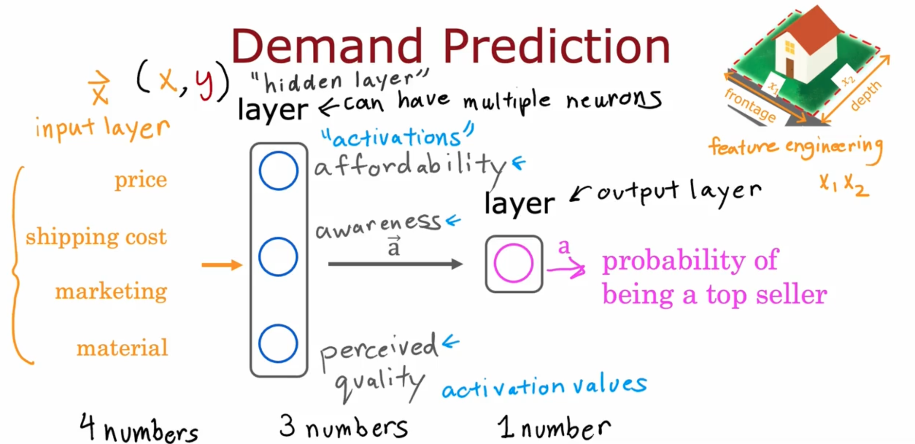The above image consists:

1. Input Layer (Represents features used to predict demand)
2. Hidden Layer (Contains neurons (nodes/units) that perform internal computation and generate activations)
3. Output Layer (Produces the final prediction output)

Neural Network Process

1. Input features → feed into hidden layer.
2. Hidden layer computes activations using learned weights.
3. Activations → passed to output layer.
4. Output layer generates final prediction (e.g., probability).

Neural Network Model

Neural Network Layer

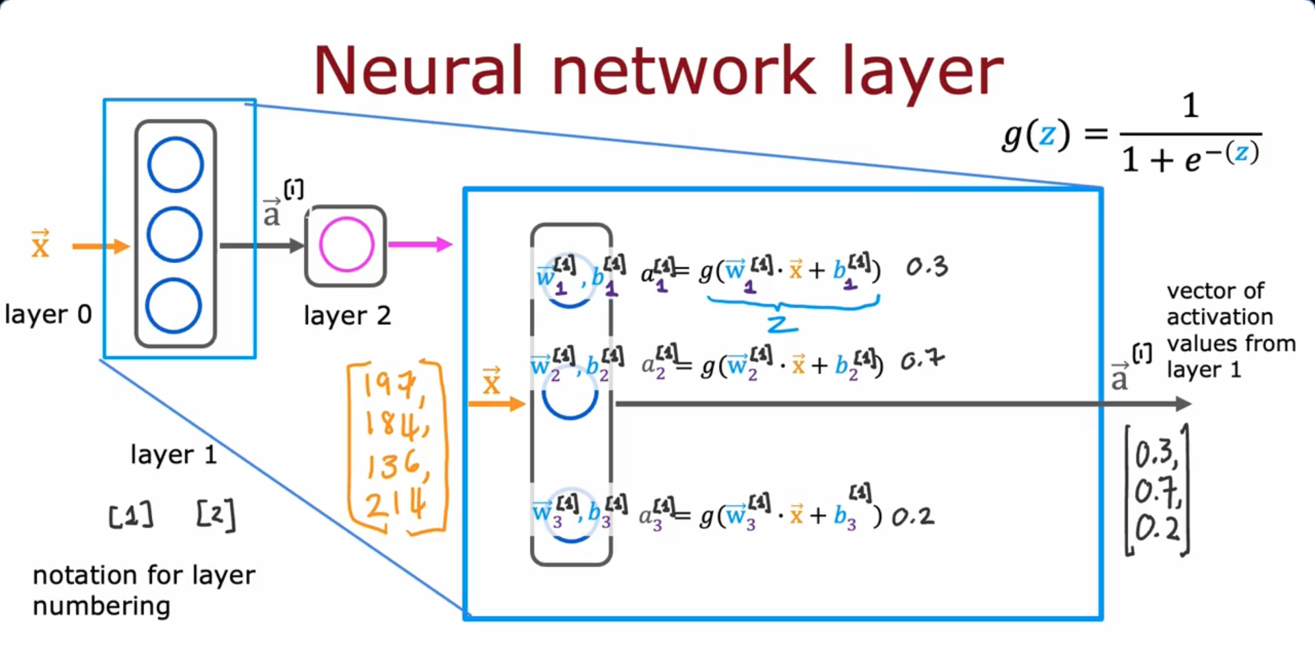
• The above figure shows the expansion of a hidden layer (layer 1), with the naming conventions, ways to write the parameters, outputs to the respective layers (We can say that there are two layers in the above neural network, we usually don’t include the input layer)
• The input and output layers are classified as layer 0 and layer 2 in the above diagram
• Each neuron of the layer 1 perform logistic regression and give outputs which are then combined to output activation vector which is given as an input to the output layer
• The output layer again performs logistic regression with the activation vector to give the layer 2 output activation vector with which we can do our inference (By using a decision boundary/ threshold)
• Since the computation goes from left to right, this algorithm is also called Forward Propagation. However the Gradient Descent uses Back Propagation to calculate derivatives

Activation value of layer l, unit(neuron) j

$$a_j^{[l]}=g\left(w_j^{[l]}\cdot a^{[l-1]}+b_j^{[l]}\right)$$ $$\text{where:}$$ $$a_j^{[l]}=\text{activation value of unit }j\text{ in layer }l$$ $$w_j^{[l]}=\text{weight vector of unit }j\text{ in layer }l$$ $$a^{[l-1]}=\text{activation vector from layer }l-1$$ $$b_j^{[l]}=\text{bias of unit }j\text{ in layer }l$$ $$g(\cdot )=\text{activation function (e.g., sigmoid, ReLU)}$$

Neural Network Training

Tensorflow code

import tensorflow as tf
from tensorflow.keras import Sequential
from tensorflow.keras.layers import Dense
 
# STEP 1 - Specifies architecture of the neural network
model = Sequential([
	Dense(units=25, activation='sigmoid'),
	Dense(units=15, activation='sigmoid'),
	Dense(units=1, activation='sigmoid'),
])
 
# STEP 2 - Loss and cost functions (Logistic loss -> Binary Cross Entropy)
# Incase we have a regression problem, we can use (loss -> MeanSquaredError())
 
from tensorflow.keras.losses import BinaryCrossentropy
model.compile(loss=BinaryCrossentropy())
 
 
# STEP 3 - Gradient descent to minimize the cost function (Also computes derivatives for gradient descent using "back propagation")
 
model.fit(X,Y, epochs=100) #epochs refer to number of steps in gradient descent

Activation Functions

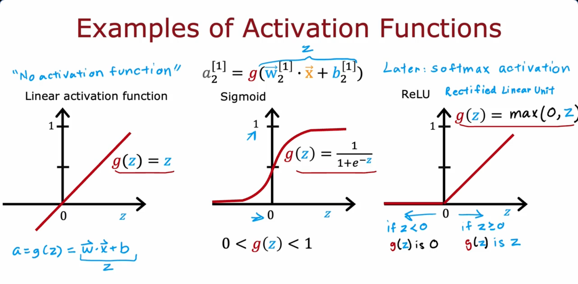
Mostly commonly used Activation functions :

1. Linear Activation Function - Preferred fro Regression
2. Sigmoid - Preferred for binary classification
3. ReLU (Rectified Linear Unit) - To get any positive value as output. Has lower Computational Cost, faster Convergence Speed

Choosing Activation Functions

Output Layer

• Need to choose depending on what the target of ground truth label y
• Binary Classification problem → Sigmoid activation function
• Regression (Positive or Negative output values) → Linear Activation Function
• Regression (Need only non-negative output value) → ReLU

Hidden Layer

• ReLU Activation Function is the most common choice - Faster Learning
• Apart from computation speed, another reason to prefer ReLU over Sigmoid activation function is because of the fact that ReLU activation function is completely flat in one side of the graph whereas the Sigmoid activation function goes flat in two places (To the left and right of the graph)
• When we use Gradient descent to train a neural network, when there is a function that is flat in a lot of places, Gradient descent would be very slow

Why do we need Activation Functions ?

• Let’s assume we use the Linear activation function in all the hidden layers and the output layer - > This would eventually result in Linear Regression
• Let’s assume we use the Linear activation function in all the hidden layers and Sigmoid activation function in the output layer → This would eventually result in Logistic Regression
• Both the above cases fail to use the potential of the entire neural network model

Multi-class Classification

Classification problems with more than two possible output labels

Softmax

Generalization of logistic regression to the multi-class classification context

Softmax Regression (4 possible outputs, example)

$$z_1={\vec{w}}_1\cdot \vec{x}+b_1$$ $$a_1=\frac{e^{z_1}}{e^{z_1}+e^{z_2}+e^{z_3}+e^{z_4}}=P(y=1\mid \vec{x})=0.30$$ $$z_2={\vec{w}}_2\cdot \vec{x}+b_2$$ $$a_2=\frac{e^{z_2}}{e^{z_1}+e^{z_2}+e^{z_3}+e^{z_4}}=P(y=2\mid \vec{x})=0.20$$ $$z_3={\vec{w}}_3\cdot \vec{x}+b_3$$ $$a_3=\frac{e^{z_3}}{e^{z_1}+e^{z_2}+e^{z_3}+e^{z_4}}=P(y=3\mid \vec{x})=0.15$$ $$z_4={\vec{w}}_4\cdot \vec{x}+b_4$$ $$a_4=\frac{e^{z_4}}{e^{z_1}+e^{z_2}+e^{z_3}+e^{z_4}}=P(y=4\mid \vec{x})=0.35$$

Softmax Regression (N possible outputs: y = 1, 2, 3, …, N)

$$z_j={\vec{w}}_j\cdot \vec{x}+b_j\text{for }j=1,2,\dots ,N$$ $$a_j=\frac{e^{z_j}}{{\sum }_{k=1}^N{e}^{z_k}}=P(y=j\mid \vec{x})$$ $$\text{Note: }{a}_1+a_2+\cdots +a_N=1$$

Cost Function

Softmax Regression

$$a_1=\frac{e^{z_1}}{e^{z_1}+e^{z_2}+\cdots +e^{z_N}}=P(y=1\mid \vec{x})$$ $$⋮$$ $$a_N=\frac{e^{z_N}}{e^{z_1}+e^{z_2}+\cdots +e^{z_N}}=P(y=N\mid \vec{x})$$

Cross-Entropy Loss Function

$$\text{loss}(a_1,\dots ,a_N,y)=\{\begin{array}{ll}-\log a_1& \text{if }y=1\\ -\log a_2& \text{if }y=2\\ ⋮& \\ -\log a_N& \text{if }y=N\end{array}$$ $$\text{loss}=-\log a_j\text{if }y=j$$

Tensor Flow Implementation - Softmax

This is the code to solve Multi-class classification problem

model = Sequential([
	Dense(units=25, activation='relu'),
	Dense(units=15, activation='relu'),
	Dense(units=10, activation='softmax')
	])
	
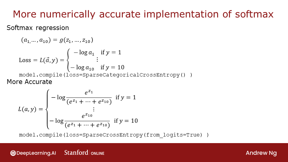
model.compile(loss=SparseCategoricalCrossEntropy())

The following code does the same calculations as the previous code, but is more numerically accurate (Referred to as “Numerical roundoff errors” )

model = Sequential([
	Dense(units=25, activation='relu'),
	Dense(units=15, activation='relu'),
	Dense(units=10, activation='linear') #softmax is replaced with linear
	])
	
model.compile(loss=SparseCategoricalCrossEntropy(from_logits=True))
 
model.fit(X, Y, epochs=100)
 
logits = model(X) #The final neural network layer no longer outputs probabilities a1...a0. Insetead it outputs z1....z10. 
 
f_x = tf.nn.softmax(logits) #Hence, we pass it through the softmax function in order to get the probability

Multi-label Classification

• Given an input image, the model has to predict if the specified elements are present or not
• To achieve this, we can design a neural network where the Output layer consists of three sigmoid activation units. With the output layer, we’ll get y as the output

$$\text{Image 1:}y=\left[\begin{array}{c}1\\ 0\\ 1\end{array}\right]\begin{array}{rl}\text{Is there a car?}& \text{yes}\\ \text{Is there a bus?}& \text{no}\\ \text{Is there a pedestrian?}& \text{yes}\end{array}$$ $$\text{Image 2:}y=\left[\begin{array}{c}0\\ 0\\ 1\end{array}\right]\begin{array}{rl}\text{Is there a car?}& \text{no}\\ \text{Is there a bus?}& \text{no}\\ \text{Is there a pedestrian?}& \text{yes}\end{array}$$ $$\text{Image 3:}y=\left[\begin{array}{c}1\\ 1\\ 0\end{array}\right]\begin{array}{rl}\text{Is there a car?}& \text{yes}\\ \text{Is there a bus?}& \text{yes}\\ \text{Is there a pedestrian?}& \text{no}\end{array}$$

Advanced Optimization

There are a few algorithms for optimization (Reducing Cost function) that are better than Gradient Descent

Adam (Adaptive Moment estimation) Algorithm

• Increase α - During the gradient descent process, if the next consecutive steps are being taken in the same direction, one small step at a time, the algorithm finds it and increases the learning rate value
• Decrease α - Similarly, if we have initialized the learning rate to a bigger value during the stat of the gradient descent and because of this the next steps are too deviated, hence the algorithm decreases the learning rate value

Code : The initial learning_rate is passed to the code

mode.compile(optimizer=tf.keras.optimizers.Adam(learning_rate=1e-3),
  loss=tf.keras.losses.SparseCategoricalCrossentropy(from_logits=True))

Additional Layer Types

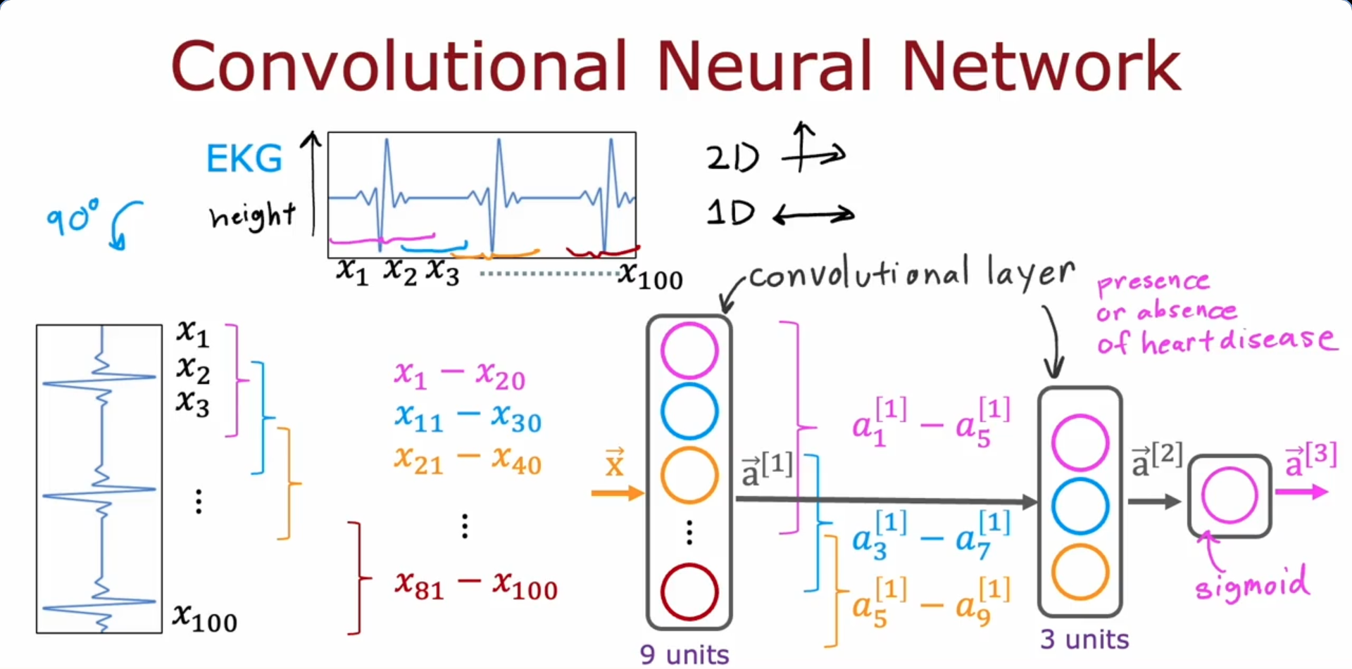
Dense Layer : Each neuron output is a function of all the activation outputs of the previous layer

Convolutional Layer : Each neuron only looks at part of the previous layer’s outputs

• Faster computation
• Need less training data (Less prone to overfitting)

Advice for applying Machine Learning

Evaluating a model

Train-Test split

• Split the dataset into two parts, the Training set(70%) and Testing set(30%)
• We find the parameters by minimizing cost function for the training set
• Then, we compute the test error (squared error cost) to find how well the training data has trained the model
• Problem with this method : The test error is likely to be an optimistic estimate of the generalization error. The model may not work properly when a new data is input for it to calculate/ classify

Model Selection and training/cross validation/test sets

Train - Cross Validation - Test split

• Split the dataset into three parts, the Training set(60%), Cross validation set(20%) and Testing set(20%)
• We find the parameters by minimizing cost function for the training set

We train models of increasing complexity (polynomial degree $d$):

$$d=1:f_{\vec{w},b}(\vec{x})=w_{1}x+b$$ $$d=2:f_{\vec{w},b}(\vec{x})=w_{1}x+w_2{x}^2+b$$ $$d=3:f_{\vec{w},b}(\vec{x})=w_{1}x+w_2{x}^2+w_3{x}^3+b$$ $$⋮$$ $$d=10:f_{\vec{w},b}(\vec{x})=w_{1}x+w_2{x}^2+\cdots +w_{10}{x}^{10}+b$$

Evaluate each model on the cross-validation set:

$$J_{cv}(w^{⟨1⟩},b^{⟨1⟩}),J_{cv}(w^{⟨2⟩},b^{⟨2⟩}),\dots ,J_{cv}(w^{⟨10⟩},b^{⟨10⟩})$$

Choose the model with the lowest cross-validation error. Suppose it’s $d=4$:

$$\text{Pick:}{f}_{\vec{w},b}(\vec{x})=w_{1}x+w_2{x}^2+w_3{x}^3+w_4{x}^4+b$$ $$\text{Model chosen based on: }{J}_{cv}(w^{⟨4⟩},b^{⟨4⟩})$$

Estimate generalization error using the test set:

$$J_{test}(w^{⟨4⟩},b^{⟨4⟩})$$

Bias and Variance

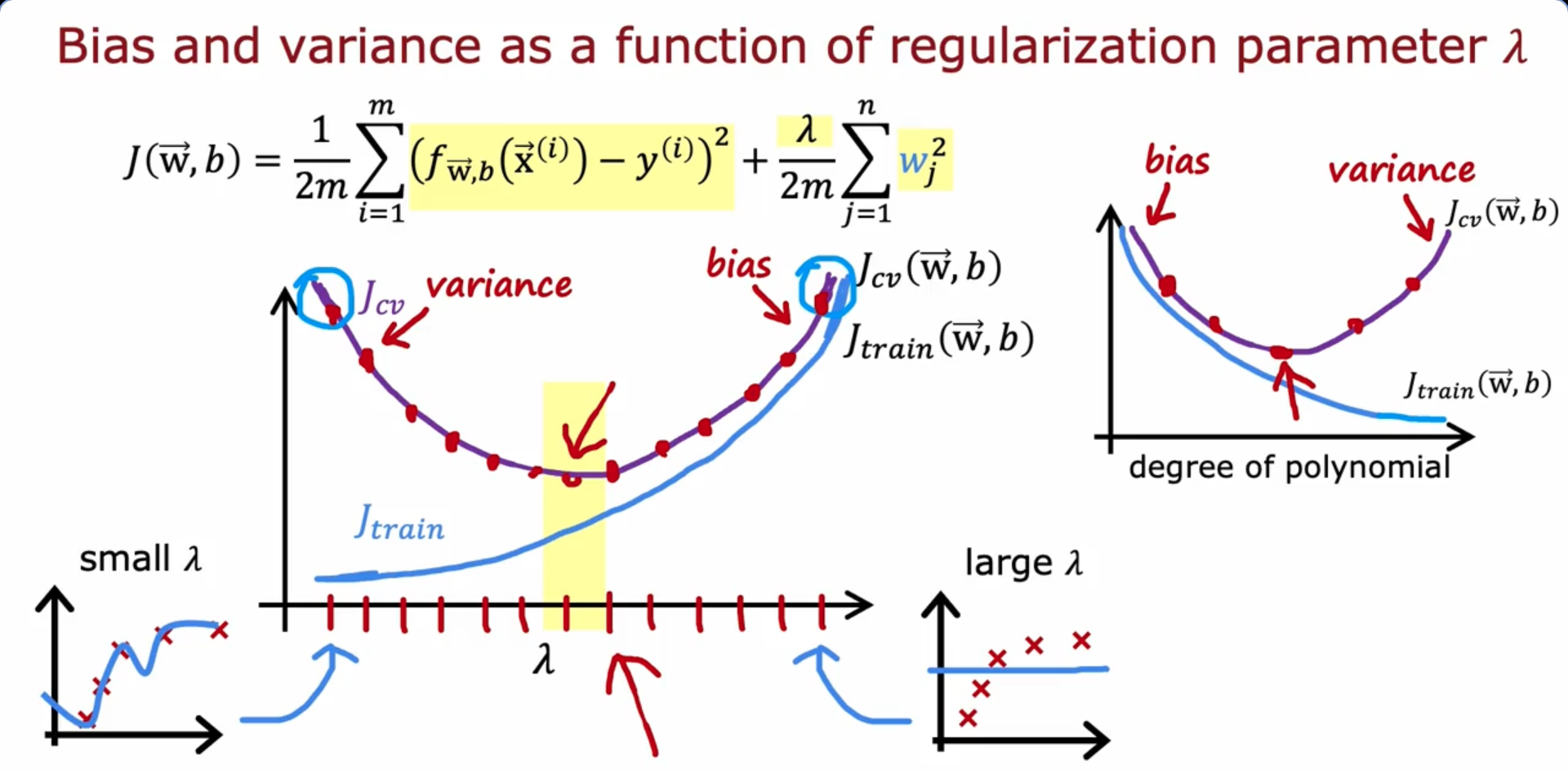
Regularization and bias/ variance

• A very high lambda(λ) value would make the parameter w to be of a very low value (~0) thus causing high bias/ under-fitting
• A very low lambda(λ) value would mean minimum regularization causing high variance/ over-fitting

Establishing a baseline level of performance

What is the level of error we can reasonably hope to get to ?

• Human level performance
• Competing algorithms performance
• Guess based on experience

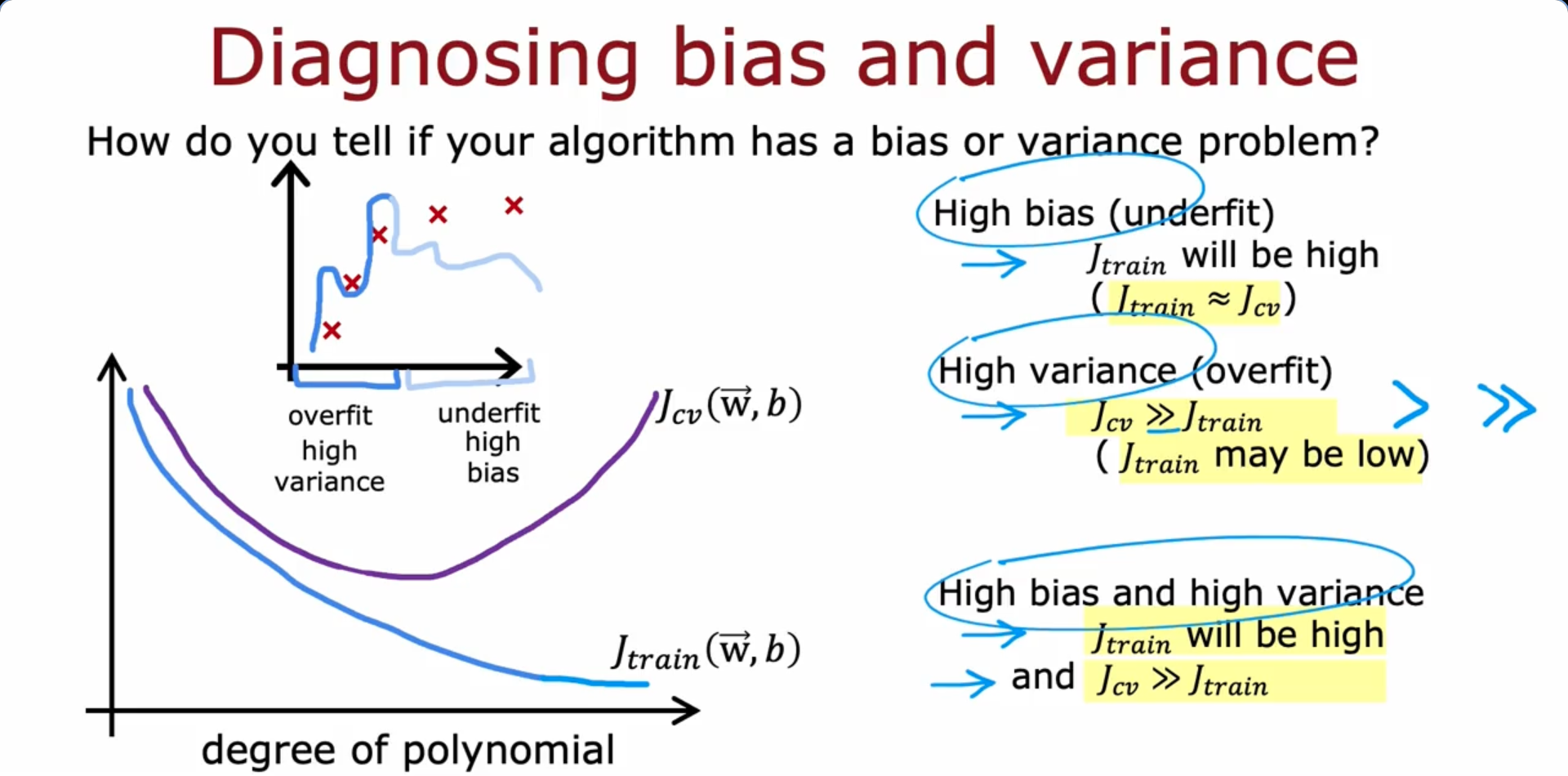
Case 1: High Variance

• Baseline Error: 10.6%
• Training Error (J_train): 10.8%
• Validation Error (J_cv): 14.8%
• Train - Baseline Gap: 0.2%
• Validation - Train Gap: 4.0%
• Diagnosis: High Variance

Case 2: High Bias

• Baseline Error: 10.6%
• Training Error (J_train): 15.0%
• Validation Error (J_cv): 15.5%
• Train - Baseline Gap: 4.4%
• Validation - Train Gap: 0.5%
• Diagnosis: High Bias

Case 3: High Bias + High Variance

• Baseline Error: 10.6%
• Training Error (J_train): 15.0%
• Validation Error (J_cv): 19.7%
• Train - Baseline Gap: 4.4%
• Validation - Train Gap: 4.7%
• Diagnosis: High Bias and High Variance

Learning Curves

• If a learning algorithm suffers from high bias, getting more training data will not (by itself) help much
• If a learning algorithm suffers from high variance, getting more training data is likely to help

We’ve implemented regularized linear regression on housing prices:

$$J(\vec{w},b)=\frac{1}{2m}\sum _{i=1}^m{\left(f_{\vec{w},b}({\vec{x}}^{(i)})-y^{(i)}\right)}^2+\frac{\lambda }{2m}\sum _{j=1}^n{w}_j^2$$

But it makes unacceptably large errors in predictions. What do we try next?

Possible Fixes and What They Address

1. Get more training examples
   Fixes: High Variance
2. Try smaller sets of features
   Fixes: High Variance
3. Try getting additional features
   Fixes: High Bias
4. Try adding polynomial features (e.g., (x_1^2, x_2^2, x_1 x_2, …))
   Fixes: High Bias
5. Try decreasing (λ)
   Fixes: High Bias
6. Try increasing (λ)
   Fixes: High Variance

Bias/ variance and neural networks

• Large neural networks are low bias machines
• A large neural network will usually do as well or better than a smaller one so long as regularization is chosen appropriately (Though it may slow down the performance of the algorithm)

Un-regularized MNIST model

layer_1 = Dense(units=25, activation="relu")
layer_2 = Dense(units=15, activation="relu")
layer_3 = Dense(units=1, activation="sigmoid")
model = Sequential([layer_1, layer_2, layer_3])

Regularized MNIST model

layer_1 = Dense(units=25, activation="relu", kernel_regularizer=L2(0.01))
layer_2 = Dense(units=15, activation="relu", kernel_regularizer=L2(0.01))
layer_3 = Dense(units=1, activation="sigmoid", kernel_regularizer=L2(0.01))
model = Sequential([layer_1, layer_2, layer_3])

Machine Learning Development Process

Iterative loop of ML development

1. Choose architecture (model, data , etc.)
2. Train model
3. Diagnostics (bias, variance and error analysis) Let’s take the example of spam classifier, try the following methods to reduce the error:

• Collect more data. E.g., “honeypot” project
• Develop sophisticated features based on email routing (From email header)
• Define sophisticated features from email body. E.g., should “discounting” and “discount” be treated as the same word
• Design algorithms to detect misspellings. E.g., w4tches, med1cine, m0rtgage

Error analysis

• Second important task after figuring out bias and variance diagnostics
• In case the algorithm misclassifies a lot, a manual examination might be needed for the fix

Adding data

• Add more data of the types where error analysis has indicated it might help (Instead of adding more data of everything)
• Data Augmentation: Modifying an existing training example to create a new training example (The distortion introduced should be representation of the type of noise/distortions in the test set. Usually doesn’t help to add purely random/meaningless noise to our data)
• Data Synthesis : Using artificial data inputs to create a new training example (Brand new)

Engineering the data used by our system : AI = Code (algorithm/model) + Data

• Conventional model-centric approach : Initially, people were focusing mostly on the Code to enhance the model/algorithm performance
• Data-centric approach : Now that the algorithms have themselves become much better in performance (Neural Networks for example), people are now focusing on Data (Such as Data Engineering, collecting more data, Data Augmentation etc.). This could be an efficient way to improve the performance of algorithm

Transfer Learning

For an application where we don’t have enough data, transfer learning is a technique that allows to use data from a different task to help on our application. However, the supervised pre-training model’s input and the fine-tuning model’s input should be of same type

Option 1 (Very small Training set): Only train output layers parameters Option 2 (Training set with enough data): Train all parameters (However, except for the output layer, the parameters would be initialized from values trained from the previous model for the respective layers)

1. Download neural network parameters pre-trained on a large dataset with same input type (e.g., images, audio, text) as our application (or train our own)
2. Further train (fine tune) the network on our own data

Full cycle of a machine learning project

1. Scope project
   → Define project goals and problem statement.

2. Collect data
   → Define what data is needed and collect relevant datasets.

3. Train model
   → Training, error analysis, and iterative improvement.

4. Deploy in production
   → Deploy the model, monitor its performance, and maintain the system.

Iterative loops may occur between:

• Deployment ↔ Training (for performance improvements)
• Training ↔ Data Collection (for better features or more data)

Deployment

		-----------------------      API call (x)       -------------------
		|   Inference Server. |   <-----------------    |                 |
		|  ------------------ |       (audio clip)      |    Mobile app   |
		|  |    ML Model    | |                         |                 |
		|  ------------------ |      Inference (ŷ)      -------------------
		|                     |   ------------------>
		-----------------------    (text transcript)

Software Engineering may be needed for (MLOps - Machine Learning Operations):

1. Ensure reliable and efficient predictions
2. Scaling
3. Logging
4. System monitoring
5. Model updates

Fairness, bias and ethics

Bias

• Hiring tool that discriminates against women
• Facial recognition system matching dark skinned individuals to criminal mugshots
• Biased bank loan approvals against sub groups
• Toxic effect of reinforcing negative stereotypes

Negative use cases

• Deepfakes
• Generating fake content for commercial or political purposes
• Using ML to build harmful products, commit fraud etc.

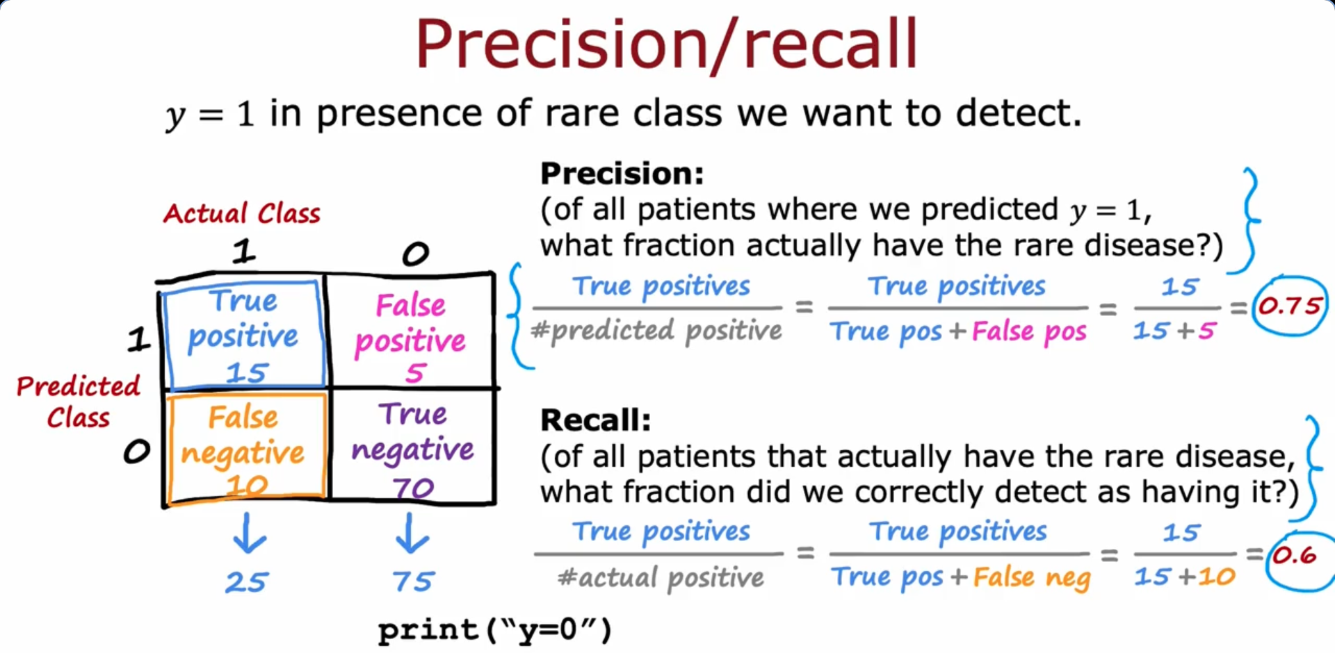
Precision/ recall

F1 score formula The F1 score is a metric used to evaluate the performance of a classification model, especially in imbalanced/skewed datasets. It is the harmonic mean of precision and recall.

$$F_1=2\cdot \frac{\text{Precision}\cdot \text{Recall}}{\text{Precision}+\text{Recall}}$$ $$\text{Precision}=\frac{\text{TP}}{\text{TP}+\text{FP}},\text{Recall}=\frac{\text{TP}}{\text{TP}+\text{FN}}$$

Decision Trees

• Features are Categorical (discrete values)

1. Root node
2. Decision Nodes
3. Leaf nodes

Decision Tree Learning - Question

Decision 1 : How to choose what feature to split on at each node ? Decision 2 : When do we stop splitting ?

Measuring Purity

Entropy as a measure of impurity

$$p_0=1-p_1$$ $$H(p_1)=-p_1{\log }_2(p_1)-p_0{\log }_2(p_0)$$ $$=-p_1{\log }_2(p_1)-(1-p_1){\log }_2(1-p_1)$$

p1 = 0 (All Dogs) Entropy = H(p1) = 0

p1 = 2/6 (2 Cats, 4 Dogs) Entropy = H(p1) = 0.92

p1 = 3/6 (3 Cats, 3 Dogs) Entropy = H(p1) = 1

p1 = 5/6 (5 Cats, 1 Dog) Entropy = H(p1) = 0.65

p1 = 6/6 (All Cats) Entropy =** H(p1) = 0

• The impurity decreases, purity increases as we go from 50-50 mix of cats and dogs to 100% all cats
• Node with a lot of examples and high entropy is worse than a node with few examples and high entropy

Choosing a split: Information Gain

Information Gain : Reduction of entropy

$$\text{Information Gain}=H(p_1^{\text{root}})-\left(w^{\text{left}}H(p_1^{\text{left}})+w^{\text{right}}H(p_1^{\text{right}})\right)$$

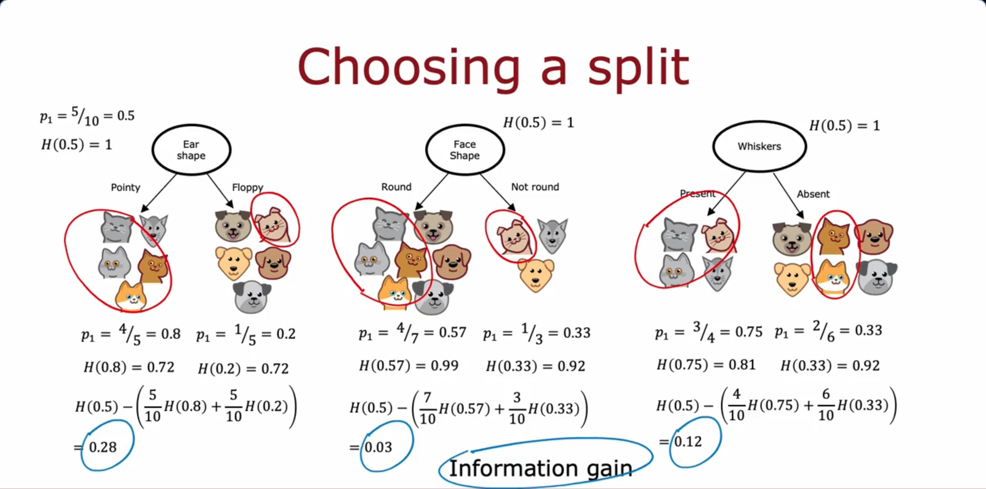
Decision Tree Learning - Answer (Recursive algorithm)

• Start with all examples at the root node
• Calculate information gain for all possible features, and pick the one with the highest information gain
• Split dataset according to selected feature, and create left and right branches
• Keep repeating splitting process until stopping criteria is met:
  • When a node is 100% one class
  • When splitting a node will result in the tree exceeding a maximum depth (Very large value for depth might result in over-fitting)
  • When improvements in purity score are below a threshold
  • When number of examples in a node is below a threshold

Using one-hot encoding of categorical features

• One hot encoding : If a categorical feature can take on k values, create k binary features (0 or 1 valued)

Continuous valued features

• Take a few threshold values to classify between the given output labels. Calculate the Information gain for the values, compare them with the Information gain of other features as well and choose the split accordingly

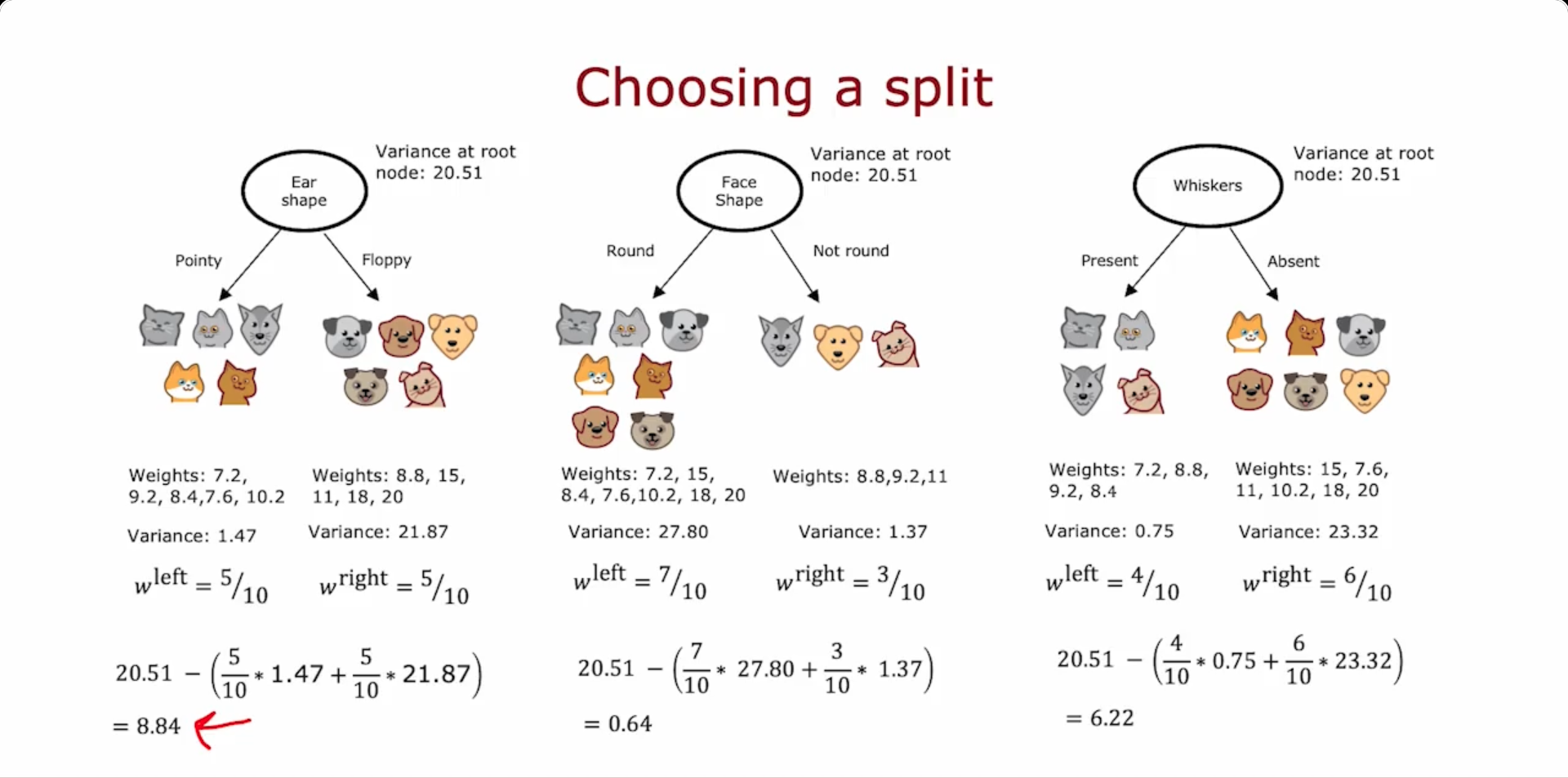
Regression Trees

• Focus on the reduction in variance to choose the split

Tree Ensembles

Using multiple decision trees

Using a single decision tree has the weakness of being sensitive to small change sin the data. Thus, building a lot of decision tree’s (ensemble) is more robust

Sampling With replacement

• Helps to construct a new training set that’s a bit similar to but still different from the original training set (This will be the key building block for building an ensemble of tree)

Random Forest Algorithm

Powerful tree ensemble algorithm

Given training set of size m For b = 1 to B: Use sampling with replacement to create a new training set of size m Train a decision tree on the new dataset

• B can typically take value of 64-128
• During the decision, we take all the tree results to vote

Random forest algorithm :

• At each node, when choosing a feature to use to split, if n features are available, pick a random subset of k < n features and allow the algorithm to only choose from that subset of features (k = √n typically for larger k values)

XGBoost (eXtreme Gradient Boosting)

Open-source, runs faster, most widely used, has built in regularization to prevent overfitting

Given training set of size m For b = 1 to B: Use sampling with replacement to create a new training set of size m (But, instead of picking from all examples with equal (1/m) probability, make it more likely to pick misclassified examples from previously trained trees) Train a decision tree on the new dataset

from xgboost import XGBClassifier
 
model = XGBClassifier()    #XGBRegressor() for Regression problem
 
model.fit(X_train, y_train)
y_pred = model.predict(X_test)

When to use decision trees

Decision Trees and Tree ensembles

• Works well on tabular (structured) data (Data stored in spreadsheet)
• Not recommended for unstructured data (images, audio, text)
• Fast
• Small decision trees may be human interpretable

Neural Networks

• Works well on all types of data, including tabular (structured) and unstructured data
• May be slower than a decision tree
• Works with transfer learning
• When building a system of multiple models working together, it might be easier to string together multiple neural networks