Supervised Machine Learning - Regression and Classification

ML is the field of study that gives computers the ability to learn without being explicitly programmed

Supervised vs. Unsupervised Machine Learning

Supervised Learning

  x         ----->      y
input              output label

Learns from being given “right answers” (We provide enough examples with input x along with corresponding output label y from which the machine learns. Eventually, when we give an new input without output label, it’ll generate the output by itself based on the learning)

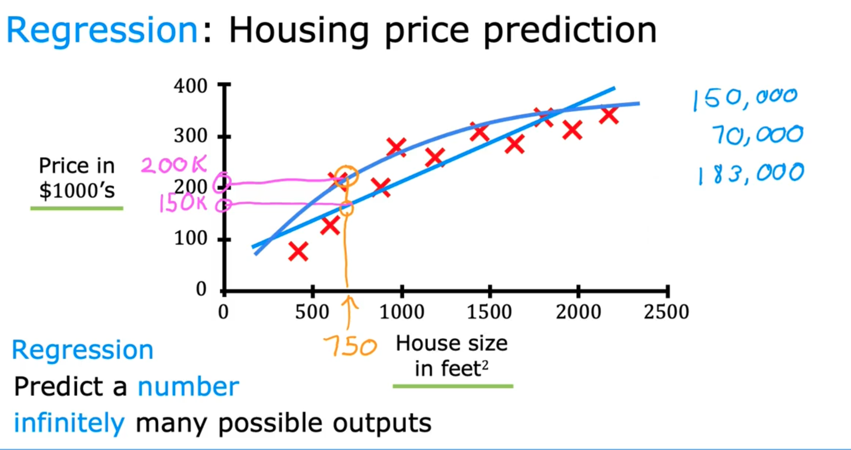
Regression

Type of Supervised Learning that predicts a number (There could be infinitely many possible outputs)

Housing price prediction (Given a set of House size with the corresponding Price for it, we make the algorithm to fit a curve along the given points, now when we need the price for a new house with a randomly input House size, we can get the value from the point of intersection of the curve)

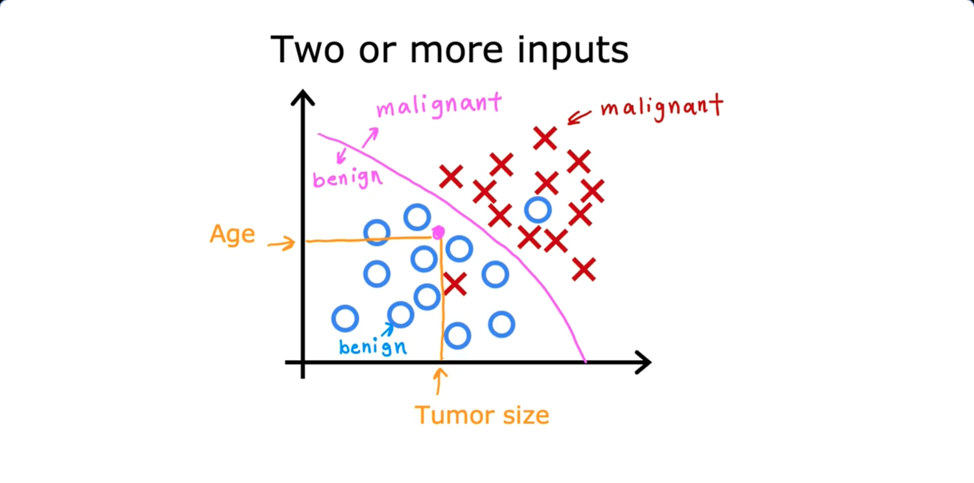
Classification

We use classification to predict only a small number of possible outcomes/ categories (Ex: Predict if a tumor is malignant or benign based on it’s size)

• Classification predict categories (Cat or Dog; Benign or Malignant; 0 or 1 or 2). The learning algorithm sets a boundary line for the given data for classification

Unsupervised Learning

Find something interesting in unlabeled data (We only provide input x, not output labels y). We let the algorithm to search for a structure in the input data

Clustering

The algorithm groups the unlabeled similar input data into clusters.>

Following are some examples:

1. Google News (Clustering of similar news)
2. DNA microarray (Clustering of people with similar DNA characteristics)

Anomaly Detection

Find unusual data points

Dimensionality Reduction

Compress data using fewer numbers

Regression Model

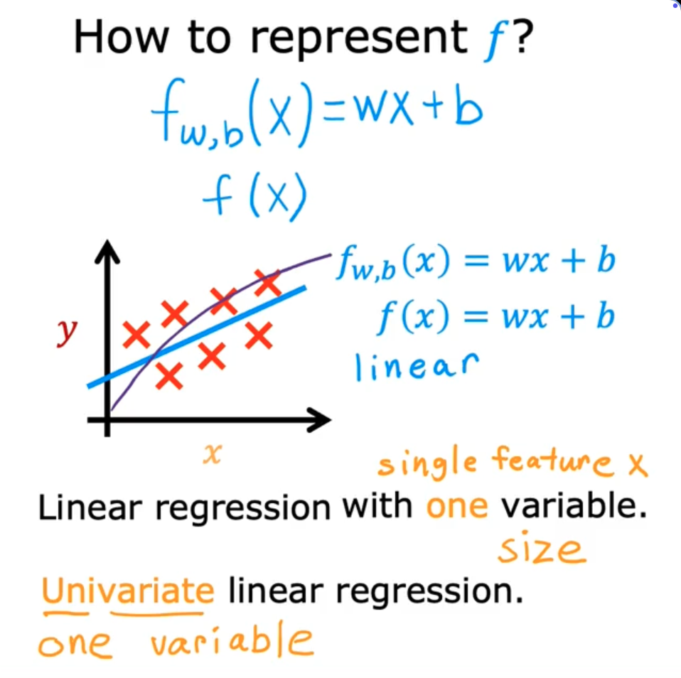
Linear Regression Model

This is a Supervised learning model. Linear regression is one of the regression models. Predicts numbers

Terminology

Data used to train the model = Training Set
x = “input” variable (feature)
y = “output” variable (target)
ŷ = modles predicted value
y = true or observed value of the dependent variable
m = number of training examples
(x, y) = single training example
(x${}^i$, y${}^i$) = i^t$$^h training example

                 +-------------------+
                 |   Training Set    |
                 +-------------------+
                           |
                           v
                 +-------------------+
                 | Learning Algorithm|
                 +-------------------+
                           |
                           v
                     +----------------+
          x  ---->   |  f(x) Function |  ---->  ŷ
      (feature)      +----------------+       (prediction)

Example:

                  +-----+
size (x)  ---->   |  f  |  ---->  price (ŷ - estimated)
                  +-----+

Cost Function: Squared Error cost function

A mathematical function that measures the difference between a model’s predictions and the actual values

The cost function ( J(w, b) ) is defined as:

$$J(w,b)=\frac{1}{2m}\sum _{i=1}^m{\left({\hat{y}}^{(i)}-y^{(i)}\right)}^2$$ $${\hat{y}}^{(i)}=f_{w,b}(x^{(i)})=w{x}^{(i)}+b$$ $$y^{(i)}\text{ is the true label/output}$$ $$m\text{ is the number of training examples}$$ $$f_{w,b}(x)\text{ is the hypothesis (linear model)}$$

The goal is to find ( w, b ) such that:

$${\hat{y}}^{(i)}\approx y^{(i)}\text{for all }(x^{(i)},y^{(i)})$$

Visualizing the cost function

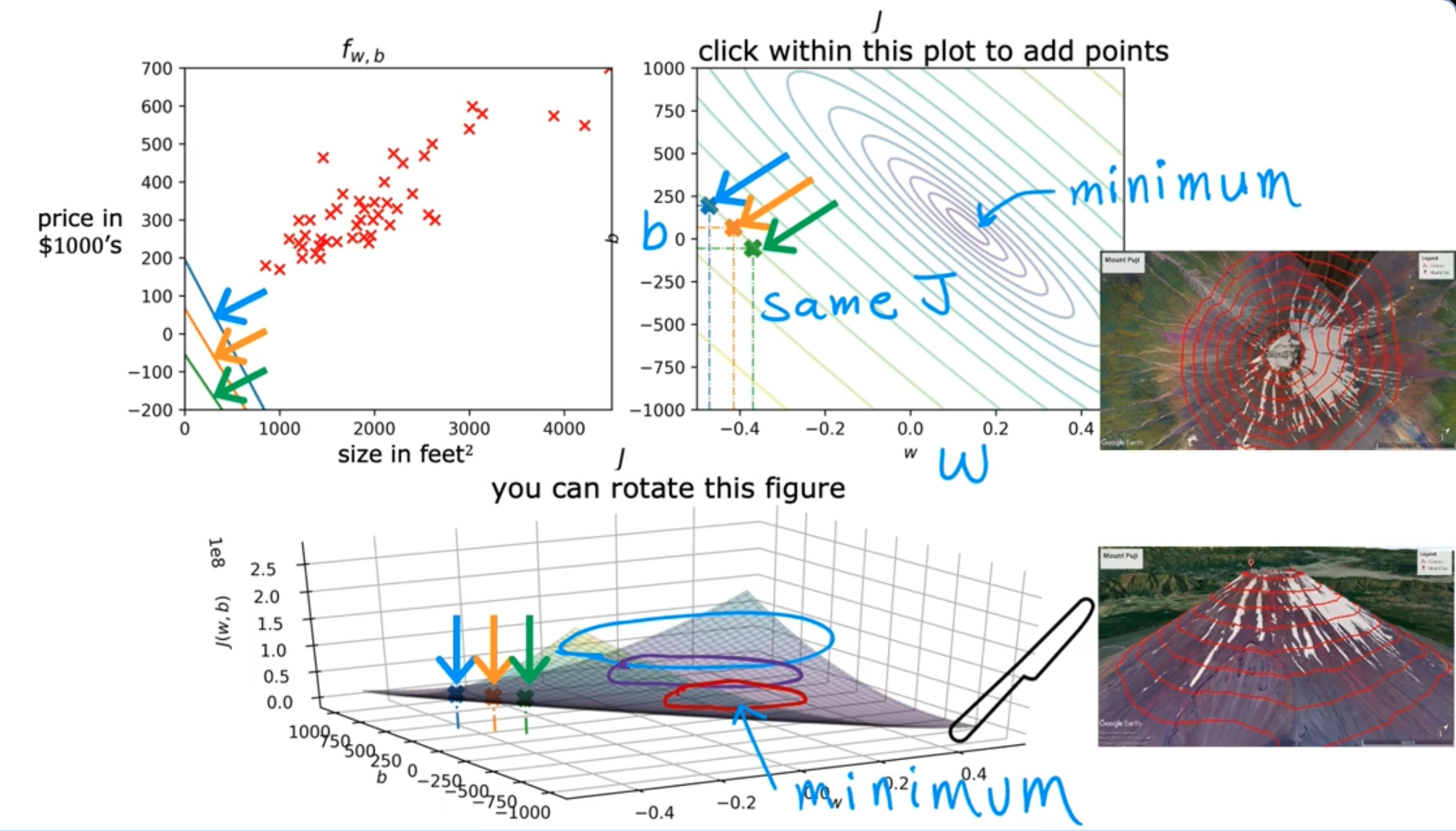
• When we represent the cost function with two input parameters (w, b) we’ll get a 3D shape
• The height of any point corresponding to w and b values will be the Cost Function value (The higher the point, higher the value of cost function)
• To represent the cost function in 2D, we use the Contour plot graph which appears to be the sliced version of the 3D plot (The smallest oval shape represents the minimum value of the Cost Function)
• For Linear Regression models, there will be only one Local Minimum ~ Global Minimum. However, for other models, there’ll be multiple local minima and the one with the lowest value will be the Global Minimum

Gradient Descent

Algorithm to minimize a function (Cost Function in our case)

• Start with some w, b (Set w=0, b=0 as the initial guess)
• Keep changing w, b to reduce J(w, b) (Simultaneously update w and b)
• Until we settle at or near a minimum
• In the algorithm below, we use Batch Gradient descent because each step of gradient descent uses all the training examples (i.e i=1 to i=m)

Gradient Descent Algorithm

Repeat until convergence:

$$w:=w-\alpha \frac{\partial }{\partial w}J(w,b)$$ $$b:=b-\alpha \frac{\partial }{\partial b}J(w,b)$$

Where:

• $\alpha$ is the learning rate
• $\frac{\partial }{\partial w}J(w,b)$ is the derivative of the cost function with respect to $w$
• $\frac{\partial }{\partial b}J(w,b)$ is the derivative of the cost function with respect to $b$

Formula after calculating the derivative Repeat until convergence:

$$w:=w-\alpha \cdot \frac{1}{m}\sum _{i=1}^m\left(f_{w,b}(x^{(i)})-y^{(i)}\right)x^{(i)}$$ $$b:=b-\alpha \cdot \frac{1}{m}\sum _{i=1}^m\left(f_{w,b}(x^{(i)})-y^{(i)}\right)$$

Where:

• $f_{w,b}(x^{(i)})=w{x}^{(i)}+b$ is the hypothesis(Models’ prediction function)
• $\alpha$ is the learning rate
• $m$ is the number of training examples
• $(x^{(i)},y^{(i)})$ is the $i^{th}$ training example

Multiple Linear Regression

Multiple Features

We represent each training example with multiple input features. Let:

$$x_j=\text{the }{j}^{\text{th}}\text{ feature}$$ $$n=\text{number of features}$$ $${\vec{x}}^{(i)}=\text{feature vector of the }{i}^{\text{th}}\text{ training example}$$ $$x_j^{(i)}=\text{value of the }{j}^{\text{th}}\text{ feature in the }{i}^{\text{th}}\text{ training example}$$

Hypothesis for Multiple Linear Regression

$$f_{\vec{w},b}(\vec{x})=w_1{x}_1+w_2{x}_2+\cdots +w_n{x}_n+b$$ $$\vec{w}=[w_1,w_2,w_3,\dots ,w_n]$$ $$b\text{ is a number}$$ $$\vec{x}=[x_1,x_2,x_3,\dots ,x_n]$$ $$\text{Compact vector form using dot product:}$$ $$f_{\vec{w},b}(\vec{x})=\vec{w}\cdot \vec{x}+b$$ $$\text{Can be expanded again to:}$$ $$f_{\vec{w},b}(\vec{x})=w_1{x}_1+w_2{x}_2+w_3{x}_3+\cdots +w_n{x}_n+b$$ $$\text{This is the hypothesis function for multiple linear regression.}$$

Vectorization

1. Makes the code shorter
2. Makes the code run much faster (NumPy library uses parallel hardware either CPU or GPU)

Let’s consider the following data

w = np.array([1.0,2.5,-3.3])
b = 4
x = np.array([10,20,30])

Code to find f(x) without vectorization (Option 1)

f = w[0] * x[0] +
	w[1] * x[1] +
	w[2] * x[2] + b

Code to find f(x) without vectorization (Option 2)

f =0
for j in range(0,n):
	f = f + w[j] * x[j]
f = f + b

Code with Vectorization

f = np.dot(w,x) + b

Gradient Descent for Multiple Linear Regression

Gradient descent now becomes as follows:

$$w:=w-\alpha \frac{\partial }{\partial w}J(\vec{w},b)$$ $$b:=b-\alpha \frac{\partial }{\partial b}J(\vec{w},b)$$ $$\text{n features }(n\ge 2)$$ $$\text{Repeat { for }j=1,\dots ,n:$$ $$w_j=w_j-\alpha \cdot \frac{1}{m}\sum _{i=1}^m\left(f_{\vec{w},b}({\vec{x}}^{(i)})-y^{(i)}\right)x_j^{(i)}$$ $$\text{Update bias:}b=b-\alpha \cdot \frac{1}{m}\sum _{i=1}^m\left(f_{\vec{w},b}({\vec{x}}^{(i)})-y^{(i)}\right)$$ $$\text{} Simultaneously update all }{w}_j\text{ for }j=1,\dots ,n\text{ and }b$$ $$\text{Where }{f}_{\vec{w},b}({\vec{x}}^{(i)})=\vec{w}\cdot {\vec{x}}^{(i)}+b$$

Alternative to gradient descent

Normal Equation

• Only for linear regression
• Solve for w, b without iterations Disadvantages

• Doesn’t generalize to other learning algorithms
• Slow when number of features is large (> 10,000) What we need to know
• Normal equation method may be used in machine learning libraries that implement linear regression
• Gradient descent is the recommended method for finding parameters w,b

Gradient Descent in Practice

Feature Scaling

• When the possible range of values of a feature is large (House size in sq. feet x1 = 300 to 2,000), it’s more likely that a good model will choose a small parameter value (w1 = 0.1)
• When the possible range of values of a feature is small (No. of bedrooms x2 = 0 to 5), it’s more likely that a good model will choose a large parameter value (w2 = 50)
• But, when we have different features that take on different range of values, it can cause gradient descent to run slowly. But, rescaling different features so that they can all take comparable range of values can speed up gradient descent computation much faster

Divide the range by max value

$$300\le x_1\le 2000\Rightarrow x_{1,\text{scaled}}=\frac{x_1}{2000}\Rightarrow 0.15\le x_{1,\text{scaled}}\le 1$$ $$0\le x_2\le 5\Rightarrow x_{2,\text{scaled}}=\frac{x_2}{5}\Rightarrow 0\le x_{2,\text{scaled}}\le 1$$ $$\text{Where }{x}_1={\text{size in feet}}^2,x_2=\text{bedrooms}$$

Mean Normalization

Feature ranges

$$300\le x_1\le 2000,0\le x_2\le 5$$

Mean values (Of all the values of the feature)

$${\mu }_1=600,{\mu }_2=2.3$$

Normalization formulas

$$x_1^{\text{normalized}}=\frac{x_1-{\mu }_1}{2000-300}\Rightarrow -0.18\le x_1^{\text{normalized}}\le 0.82$$ $$x_2^{\text{normalized}}=\frac{x_2-{\mu }_2}{5-0}\Rightarrow -0.46\le x_2^{\text{normalized}}\le 0.54$$

Labels

$$x_1={\text{size in feet}}^2,x_2=\text{bedrooms}$$

Z-score Normalization

Ranges before normalization

$$300\le x_1\le 2000,0\le x_2\le 5$$

Mean and standard deviation

$${\mu }_1=600,{\mu }_2=2.3$$ $${\sigma }_1=450,{\sigma }_2=1.4$$

Z-score formulas

$$x_1^{\text{standardized}}=\frac{x_1-{\mu }_1}{{\sigma }_1}\Rightarrow -0.67\le x_1^{\text{standardized}}\le 3.1$$ $$x_2^{\text{standardized}}=\frac{x_2-{\mu }_2}{{\sigma }_2}\Rightarrow -1.6\le x_2^{\text{standardized}}\le 1.9$$

Labels

$$x_1={\text{size in feet}}^2,x_2=\text{bedrooms}$$

Feature Engineering

Using intuition to design new features, by transforming or combining original features

• Let’s take the problem of finding price of house given two features x1(Frontage) and x2(Depth)
• We can include a third feature x3(Area) = x1(Frontage) (x) x2(Depth) to enhance the model performance

Polynomial Regression

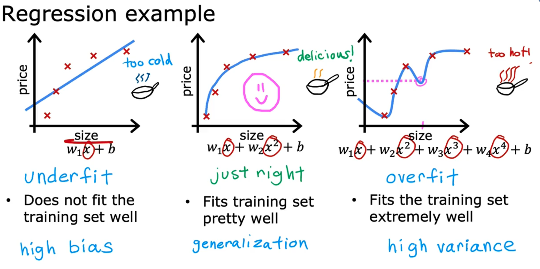
Fitting non-linear function (Curves). Given a single feature x, we can make it a quadratic, cubic equation etc. for a better fit (Gives a curve instead of a straight line model)

Quadratic Model

$$f_{\vec{w},b}(x)=w_{1}x+w_2{x}^2+b$$

Cubic Model

$$f_{\vec{w},b}(x)=w_{1}x+w_2{x}^2+w_3{x}^3+b$$

Square Root

$$f_{\vec{w},b}(x)=w_{1}x+w_2\sqrt{x}+b$$ $$\begin{gathered} \text{where:} \\ x\text{ is the input feature (e.g., size )} \\ {w}_1,w_2,w_3\text{ are the weights, } \\ b\text{ is the bias term} \end{gathered}$$

Classification with Logistic Regression

Binary classification - The output can only be one of two values(Class / Category) (e.g either yes or no)

Logistic Regression

We want outputs between 0 and 1, so we use the sigmoid (logistic) function:

$$\begin{gathered} g(z)=\frac{1}{1+e^{-z}} \\ 0<g(z)<1 \end{gathered}$$

Define:

$$z=\vec{w}\cdot \vec{x}+b$$

Then the logistic regression model is:

$$f_{\vec{w},b}(\vec{x})=g(\vec{w}\cdot \vec{x}+b)=\frac{1}{1+e^{-(\vec{w}\cdot \vec{x}+b)}}$$

---

If the logistic regression model gives a probability that the output is 1:

$$f_{\vec{w},b}(\vec{x})=\frac{1}{1+e^{-(\vec{w}\cdot \vec{x}+b)}}$$

This is interpreted as:

$$f_{\vec{w},b}(\vec{x})=P(y=1\mid \vec{x};\vec{w},b)$$

If:

$$f_{\vec{w},b}(\vec{x})=0.7$$

Then there’s a 70% chance that ( y = 1 ) (i.e., malignant).

Since this is a binary classification:

$$P(y=0)+P(y=1)=1$$

---

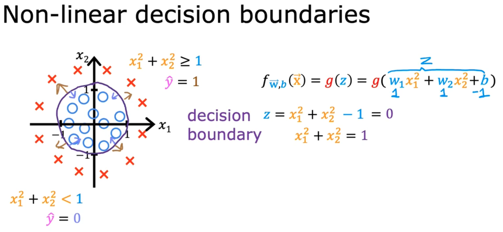
Decision Boundary

Set a threshold above which the result will be considered 1 and 0 if below

Here is how we can decide on the decision boundary:

$$f_{\vec{w},b}(\vec{x})=g(\vec{w}\cdot \vec{x}+b)=\frac{1}{1+e^{-(\vec{w}\cdot \vec{x}+b)}}$$ $$f_{\vec{w},b}(\vec{x})=P(y=1\mid \vec{x};\vec{w},b)$$ $$\hat{y}=\{\begin{array}{ll}1& \text{if }{f}_{\vec{w},b}(\vec{x})\ge 0.5\\ 0& \text{if }{f}_{\vec{w},b}(\vec{x})<0.5\end{array}$$ $$f_{\vec{w},b}(\vec{x})\ge 0.5$$ $$g(z)\ge 0.5$$ $$z\ge 0$$ $$\vec{w}\cdot \vec{x}+b\ge 0\Rightarrow \hat{y}=1$$ $$\vec{w}\cdot \vec{x}+b<0\Rightarrow \hat{y}=0$$

Cost function for Logistic Regression

• The Squared error cost function we used for Linear regression(Gives a bowl shape - convex function) doesn’t work well for Logistic Regression (Gives Non-convex graph)

Logistic Cost Function

$$J(\vec{w},b)=\frac{1}{m}\sum _{i=1}^{m}L\left(f_{\vec{w},b}({\vec{x}}^{(i)}),y^{(i)}\right)$$

Logistic Loss Function

$$L\left(f_{\vec{w},b}({\vec{x}}^{(i)}),y^{(i)}\right)=\{\begin{array}{ll}-\log \left(f_{\vec{w},b}({\vec{x}}^{(i)})\right)& \text{if }{y}^{(i)}=1\\ -\log \left(1-f_{\vec{w},b}({\vec{x}}^{(i)})\right)& \text{if }{y}^{(i)}=0\end{array}$$

Simplified Cost Function

$$L\left(f_{\vec{w},b}({\vec{x}}^{(i)}),y^{(i)}\right)=-y^{(i)}\log \left(f_{\vec{w},b}({\vec{x}}^{(i)})\right)-(1-y^{(i)})\log \left(1-f_{\vec{w},b}({\vec{x}}^{(i)})\right)$$ $$J(\vec{w},b)=\frac{1}{m}\sum _{i=1}^{m}L\left(f_{\vec{w},b}({\vec{x}}^{(i)}),y^{(i)}\right)$$ $$=-\frac{1}{m}\sum _{i=1}^m\left[y^{(i)}\log \left(f_{\vec{w},b}({\vec{x}}^{(i)})\right)+(1-y^{(i)})\log \left(1-f_{\vec{w},b}({\vec{x}}^{(i)})\right)\right]$$

Gradient Descent Implementation

$$\text{Repeat}\{\begin{array}{rl}{w}_j& =w_j-\alpha \left[\frac{1}{m}\sum _{i=1}^m\left(f_{\vec{w},b}({\vec{x}}^{(i)})-y^{(i)}\right)x_j^{(i)}\right]\\ b& =b-\alpha \left[\frac{1}{m}\sum _{i=1}^m\left(f_{\vec{w},b}({\vec{x}}^{(i)})-y^{(i)}\right)\right]\end{array}$$ $$\text{Linear regression:}{f}_{\vec{w},b}(\vec{x})=\vec{w}\cdot \vec{x}+b$$ $$\text{Logistic regression:}{f}_{\vec{w},b}(\vec{x})=\frac{1}{1+e^{-(\vec{w}\cdot \vec{x}+b)}}$$

The problem of Overfitting

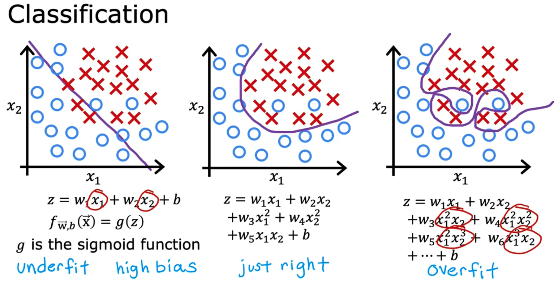
Addressing Overfitting

1. Collect more training data (The learning algorithm will learn to fit better)
2. Select features to include/ exclude (Feature selection : Choose the most relevant features)
3. Regularization (Shrink the values of parameters instead of altogether removing the features like discussed in the previous step)

Cost Function with Regularization

$$\underset{\vec{w},b}{\min }J(\vec{w},b)=\underset{\vec{w},b}{\min }\left[\frac{1}{2m}\sum _{i=1}^m{\left(f_{\vec{w},b}({\vec{x}}^{(i)})-y^{(i)}\right)}^2+\frac{\lambda }{2m}\sum _{j=1}^n{w}_j^2\right]$$

• The first term: Mean squared error (MSE) – fits the data.
• The second term: L2 regularization – penalizes large weights​ to reduce overfitting.
• lambda: Regularization strength – balances fit vs simplicity.

Regularized Linear Regression

🔹 Regularized Cost Function

$$\underset{\vec{w},b}{\min }J(\vec{w},b)=\underset{\vec{w},b}{\min }\left[\frac{1}{2m}\sum _{i=1}^m{\left(f_{\vec{w},b}({\vec{x}}^{(i)})-y^{(i)}\right)}^2+\frac{\lambda }{2m}\sum _{j=1}^n{w}_j^2\right]$$

🔹 Gradient Descent Updates

$$w_j:=w_j-\alpha \left[\frac{1}{m}\sum _{i=1}^m\left(f_{\vec{w},b}({\vec{x}}^{(i)})-y^{(i)}\right)x_j^{(i)}+\frac{\lambda }{m}{w}_j\right]$$ $$w_j:=w_j\left(1-\alpha \frac{\lambda }{m}\right)-\alpha \frac{1}{m}\sum _{i=1}^m\left(f_{w,b}({\vec{x}}^{(i)})-y^{(i)}\right)x_j^{(i)}$$

For the bias term 𝑏 (not regularized):

$$b:=b-\alpha \left[\frac{1}{m}\sum _{i=1}^m\left(f_{\vec{w},b}({\vec{x}}^{(i)})-y^{(i)}\right)\right]$$

Regularized Logistic Regression

🔹 Regularized Cost Function

$$J(\vec{w},b)=-\frac{1}{m}\sum _{i=1}^m\left[y^{(i)}\log (f_{\vec{w},b}({\vec{x}}^{(i)}))+(1-y^{(i)})\log (1-f_{\vec{w},b}({\vec{x}}^{(i)}))\right]+\frac{\lambda }{2m}\sum _{j=1}^n{w}_j^2$$

🔹 Gradient Descent Updates

$$w_j:=w_j-\alpha \left[\frac{1}{m}\sum _{i=1}^m\left(f_{\vec{w},b}({\vec{x}}^{(i)})-y^{(i)}\right)x_j^{(i)}+\frac{\lambda }{m}{w}_j\right]$$

For the bias term

$$b:=b-\alpha \left[\frac{1}{m}\sum _{i=1}^m\left(f_{\vec{w},b}({\vec{x}}^{(i)})-y^{(i)}\right)\right]$$