Unsupervised Learning, Recommenders, RL

Clustering

Looks at a number of data points and automatically finds data points that are related or similar to each other

Applications :

• Grouping similar news
• Market segmentation
• DNA analysis
• Astronomical data analysis

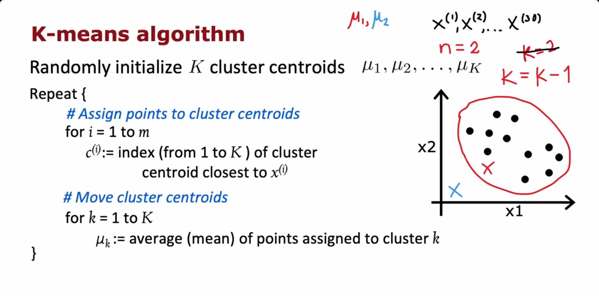
K-means Clustering algorithm

Repeatedly do:

1. Assign point to cluster centroids
2. Recompute cluster centroids (To average of all points that were assigned to it )

Optimization Objective

K - means is guaranteed to converge (On every single iteration, the distortion cost function should go down or stay the same. If it ever goes up, it means there is a bug in the code. If the value doesn’t change in the next iteration, it also means K - means has converged)

$$c^{(i)}=\text{index of cluster }(1,2,\dots ,K)\text{ to which example }{x}^{(i)}\text{ is assigned}$$ $${\mu }_k=\text{cluster centroid }k$$ $${\mu }_{c^{(i)}}=\text{cluster centroid of the cluster to which }{x}^{(i)}\text{ has been assigned}$$ $$\text{Cost function:}$$ $$J(c^{(1)},\dots ,c^{(m)},{\mu }_1,\dots ,{\mu }_K)=\frac{1}{m}\sum _{i=1}^m{\Vert x^{(i)}-{\mu }_{c^{(i)}}\Vert }^2$$ $$\underset{c^{(1)},\dots ,c^{(m)},{\mu }_1,\dots ,{\mu }_K}{\min }J(c^{(1)},\dots ,c^{(m)},{\mu }_1,\dots ,{\mu }_K)$$

Initializing K-means

Very first step of K-mean is to choose random locations as the initial guesses for the cluster centroids. How to do it best?

• Choose K < m
• Randomly pick K training examples
• Set (μ1, μ2, …, μk) the centroids equal to these K examples

$$\text{For }i=1\text{ to }100\{$$ $$\text{Randomly initialize K-means (choose }k\text{ random centroids)}$$ $$\text{Run K-means: Get }{c}^{(1)},\dots ,c^{(m)},{\mu }_1,\dots ,{\mu }_K$$ $$\text{Compute cost (distortion): }J(c^{(1)},\dots ,c^{(m)},{\mu }_1,\dots ,{\mu }_K)\}$$ $$\text{Pick the clustering with the lowest cost }J$$

Choosing the number of clusters (K)

• Often, we want to get clusters for some later (downstream) purpose
• Evaluate K-means based on how ell it performs on that later purpose

For example, in a T-shirt size clustering algorithm:

• We could have K = 3 (Three sizes - S, M, L)
• Or, we could have K = 5 (Five sizes - XS, S, M, L, XL) We need to compare both by evaluating them in the business perspective and decide which is better accordingly. For example, having 3 sizes rather than 5 has lower cost production and transportation wise. But, having 5 sizes gives a better fit for users and might satisfy them

Anomaly Detection

Given a collection of events, finding unusual events is Anomaly Detection

Gaussian (Normal) Distribution

$$p(x)=\frac{1}{\sqrt{2\pi {\sigma }^2}}{e}^{-\frac{(x-\mu {)}^2}{2{\sigma }^2}}$$ $$\begin{array}{rl}x& :\text{ A real-valued variable whose probability you’re measuring}\\ & \\ \mu & :\text{ The mean of the distribution (the peak or center of the bell curve)}\\ & \\ {\sigma }^2& :\text{ The variance, which controls how wide or narrow the bell curve is}\\ & \\ \sigma & :\text{ The standard deviation }\left(\sigma =\sqrt{{\sigma }^2}\right),\text{ representing how much variation exists from the mean}\\ & \\ \pi & :\text{ The mathematical constant }(\approx 3.14159)\end{array}$$

Mean :

$$\mu =\frac{1}{m}\sum _{i=1}^m{x}^{(i)}$$

Variance:

$${\sigma }^2=\frac{1}{m}\sum _{i=1}^m{\left(x^{(i)}-\mu \right)}^2$$

Anomaly Detection Algorithm

1. Choose n features xᵢ that we think might be indicative of anomalous examples
2. Fit parameters μ₀, μ₁,…,μ${}_n$ and σ${}_1$, σ${}_2$,…, σ${}_n$

$${\mu }_j=\frac{1}{m}\sum _{i=1}^m{x}_j^{(i)}$$ $${\sigma }_j^2=\frac{1}{m}\sum _{i=1}^m{\left(x_j^{(i)}-{\mu }_j\right)}^2$$

3. Given new example x, compute p(x):

$$p(x)=\prod _{j=1}^{n}p(x_j;{\mu }_j,{\sigma }_j^2)=\prod _{j=1}^n\frac{1}{\sqrt{2\pi }{\sigma }_j}\exp \left(-\frac{(x_j-{\mu }_j{)}^2}{2{\sigma }_j^2}\right)$$ $$\text{Anomaly if}p(x)<\epsilon$$

Developing and evaluating an anomaly detection system

Also known as real-number evaluation

• Have a few labelled data in the Cross-validation and Test sets of data. After fitting the anomaly detection model, evaluate it with the cross-validation and test sets to find out whether the algorithm is detecting the example as anomaly or not and compare this result with the label
• Use this evaluation to tune the epsilon(Threshold above which an entry is not an anomaly) value
• Can possibly consider evaluation metrics like Precision/Recall also

Anomaly Detection vs. supervised learning

Anomaly detection

• Can be preferred when having very small number of positive examples (y=1). (0-20 is common). Large number of negative (y=0) examples.
• Many different “types” of anomalies. Hard for any algorithm to learn from positive examples what the anomalies look like; future anomalies may look nothing like any of the anomalous examples we’ve seen so far
• Fraud detection
• Manufacturing - Finding new previously unseen defects in manufacturing
• Monitoring machines in a data center

Supervised Learning

• Can be preferred when having large number of positive and negative examples
• Enough positive examples for algorithm to get a sense of what positive examples are like, future positive examples likely to be similar to ones in training set
• Email spam classification
• Manufacturing - Finding known, previously seen defects
• Diseases classification

Choosing what features to use

More important task for anomaly detection

• The features must be guassian (Plotting the features should give a gaussian graph). If not, try to make them gaussian (Probably by using np.log(x) or log(x +1) or sqrt(x) etc.). These transformations makes the anomaly detection model better. Also, make sure to make the same transformation to cross-validation and testing data as well

Error analysis for anomaly detection

• Train a model, then see what anomalies in the cross-validation set that the algorithm is failing to detect. Then, look into those examples and see if that can inspire the creation of new features that would allow the model to spot that example which takes on unusually large or small value on the new features and classify whether it’s an anomaly or not

Recommender System

• System with a set of users and items (Movie ratings for example)

$$\begin{array}{rl}& \text{Notation:}\\ & \\ & r(i,j)=1\text{if user }j\text{ has rated movie }i(0\text{ otherwise})\\ & \\ & y^{(i,j)}=\text{rating given by user }j\text{ on movie }i\\ & \\ & w^{(j)},b^{(j)}=\text{parameters for user }j\\ & \\ & x^{(i)}=\text{feature vector for movie }i\\ & \\ & m^{(j)}=\text{number of movies rated by user }j\end{array}$$

---

$$\text{To learn parameters }{w}^{(j)},b^{(j)}\text{ for user }j:$$ $$J(w^{(j)},b^{(j)})=\frac{1}{2}\sum _{i:r(i,j)=1}{\left(w^{(j)}\cdot x^{(i)}+b^{(j)}-y^{(i,j)}\right)}^2+\frac{\lambda }{2}\sum _{k=1}^n{\left(w_k^{(j)}\right)}^2$$

---

$$\text{To learn parameters }{w}^{(1)},b^{(1)},w^{(2)},b^{(2)},\dots ,w^{(n_u)},b^{(n_u)}\text{ for all users:}$$ $$J\left(\begin{array}{c}{w}^{(1)},\dots ,w^{(n_u)}\\ b^{(1)},\dots ,b^{(n_u)}\end{array}\right)=\frac{1}{2}\sum _{j=1}^{n_u}\sum _{i:r(i,j)=1}{\left(w^{(j)}\cdot x^{(i)}+b^{(j)}-y^{(i,j)}\right)}^2+\frac{\lambda }{2}\sum _{j=1}^{n_u}\sum _{k=1}^n{\left(w_k^{(j)}\right)}^2$$

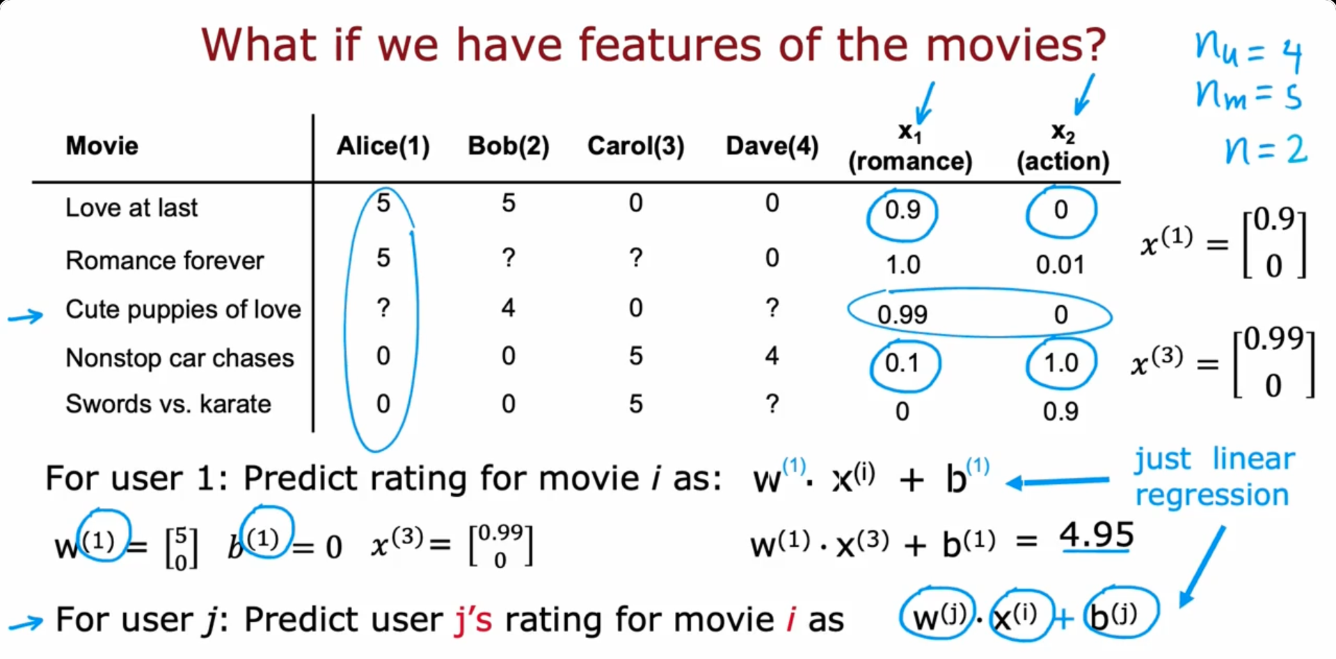
Collaborative filtering algorithm

• In the above example, we’ve got two features x${}_1$ and x${}_2$ for each movie
• In some cases, let’s say only the ratings are provided and the features aren’t given. We have to find the features ourselves

Cost function to learn w${}^j$, b${}^j$ for all users

$$\underset{w^{(1)},\dots ,w^{(n_u)},b^{(1)},\dots ,b^{(n_u)}}{\min }\frac{1}{2}\sum _{j=1}^{n_u}\sum _{i:r(i,j)=1}{\left(w^{(j)}\cdot x^{(i)}+b^{(j)}-y^{(i,j)}\right)}^2+\frac{\lambda }{2}\sum _{j=1}^{n_u}\sum _{k=1}^n{\left(w_k^{(j)}\right)}^2$$

Cost function to learn x${}^i$ for all movies

$$\underset{x^{(1)},\dots ,x^{(n_m)}}{\min }\frac{1}{2}\sum _{i=1}^{n_m}\sum _{j:r(i,j)=1}{\left(w^{(j)}\cdot x^{(i)}+b^{(j)}-y^{(i,j)}\right)}^2+\frac{\lambda }{2}\sum _{i=1}^{n_m}\sum _{k=1}^n{\left(x_k^{(i)}\right)}^2$$

Combining both together

$$\underset{\begin{array}{c}{w}^{(1)},\dots ,w^{(n_u)}\\ b^{(1)},\dots ,b^{(n_u)}\\ x^{(1)},\dots ,x^{(n_m)}\end{array}}{\min }J(w,b,x)=\frac{1}{2}\sum _{(i,j):r(i,j)=1}{\left(w^{(j)}\cdot x^{(i)}+b^{(j)}-y^{(i,j)}\right)}^2+\frac{\lambda }{2}\sum _{j=1}^{n_u}\sum _{k=1}^n{\left(w_k^{(j)}\right)}^2+\frac{\lambda }{2}\sum _{i=1}^{n_m}\sum _{k=1}^n{\left(x_k^{(i)}\right)}^2$$

We have to reduce the cost function. Gradient descent algorithm can be used for this purpose, the following are the updating steps in each iteration :

$$w_i^{(j)}=w_i^{(j)}-\alpha \frac{\partial }{\partial w_i^{(j)}}J(w,b,x)$$ $$b^{(j)}=b^{(j)}-\alpha \frac{\partial }{\partial b^{(j)}}J(w,b,x)$$ $$x_k^{(i)}=x_k^{(i)}-\alpha \frac{\partial }{\partial x_k^{(i)}}J(w,b,x)$$

Binary labels: favs, likes and clicks

Binary prediction function :

Predict that the probability of y${}^{(i,j)}$ = 1

$$f_{(w,b,x)}(x)=g\left(w^{(j)}\cdot x^{(i)}+b^{(j)}\right)$$

Binary Cross-Entropy Loss for One Example:

$$L\left(f_{(w,b,x)}(x),y^{(i,j)}\right)=-y^{(i,j)}\log \left(f_{(w,b,x)}(x)\right)-(1-y^{(i,j)})\log \left(1-f_{(w,b,x)}(x)\right)$$

Total Cost Over All Observed Ratings:

$$J(w,b,x)=\sum _{(i,j):r(i,j)=1}L\left(f_{(w,b,x)}(x),y^{(i,j)}\right)$$

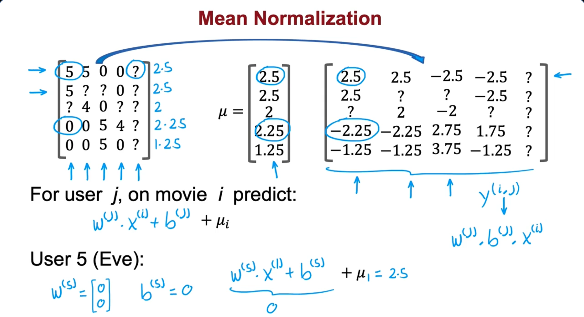
Recommender systems implementation

Mean Normalization

TensorFlow implementation

Getting the derivative term of cost function with TensorFlow

Gradient Descent

w = tf.Variable(3.0) # Tf.variables are the parameters we want to optimize
x = 1.0
y = 1.0 #target value
alpha = 0.01
 
iterations = 30
for iter in range(iterations):
   # Use TensorFlow's Gradient tape to recored the steps
   # used to compute the cost J, to enable auto differentiation.
   with tf.GradientTape() as tape:
   	fwb = w*x # Assuming b=0 for this example
   	costJ = (fwb=y)**2
 
   # Use the gradient tape to calculate the gradients
   # of the cost with respect to the parameter w.
   [dJdw] = tape.gradient(costJ, [w])
 
   # Run one step of gradient descent by updating 
   # the value of w to reduce the cost.
   w.assign_add(-alpha * dJdw) # tf.variables require special function to modify

Adam Optimizer algorithm

# Instantiate an optimizer
optimizer = keras.optimizers.Adam(learning_rate = 1e-1)
 
iterations = 200
for iter in range(iterations):
	# Use TensorFlow's GradientTape to record
	# the operations used to compute the cost
	with tf.GradientTape() as tape:
 
		# Compute the cost (forward pass is included in cost)
		cost_value = cofiCostFuncV(X, W, B, Ynorm, R,
			num_users, num_movies, lambda)
 
	# Use the gradient tape to automatically retrieve the gradients of
	# the trainable variables with respect to the loss
 
	grads = tape.gradient(cost_vale, [x,W,b])
 
	# Run one step of gradient descent by updating the 
	# value of the variables to minimize the loss.
	optimizer.apply_gradients(zip(grads, [x,W,b]))

Content-based filtering

Collaborative filtering vs Content-based filtering

Collaborative Filtering : Recommend items to you based on ratings of users who gave similar ratings as you

Content-based filtering : Recommend items to you based on features of user and item to find good match. We’ll still continue to make use of r(i, j) and y${}^{(i,j)}$

Example of the usr and movie features :

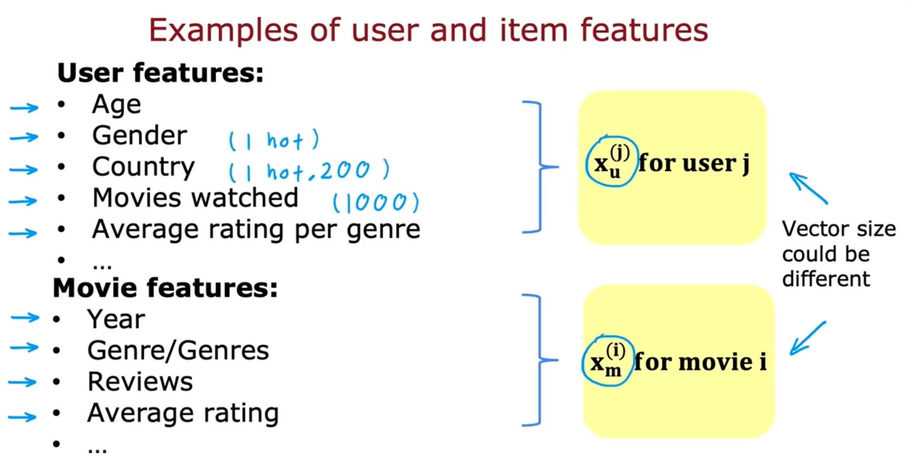
Deep learning for content-based filtering

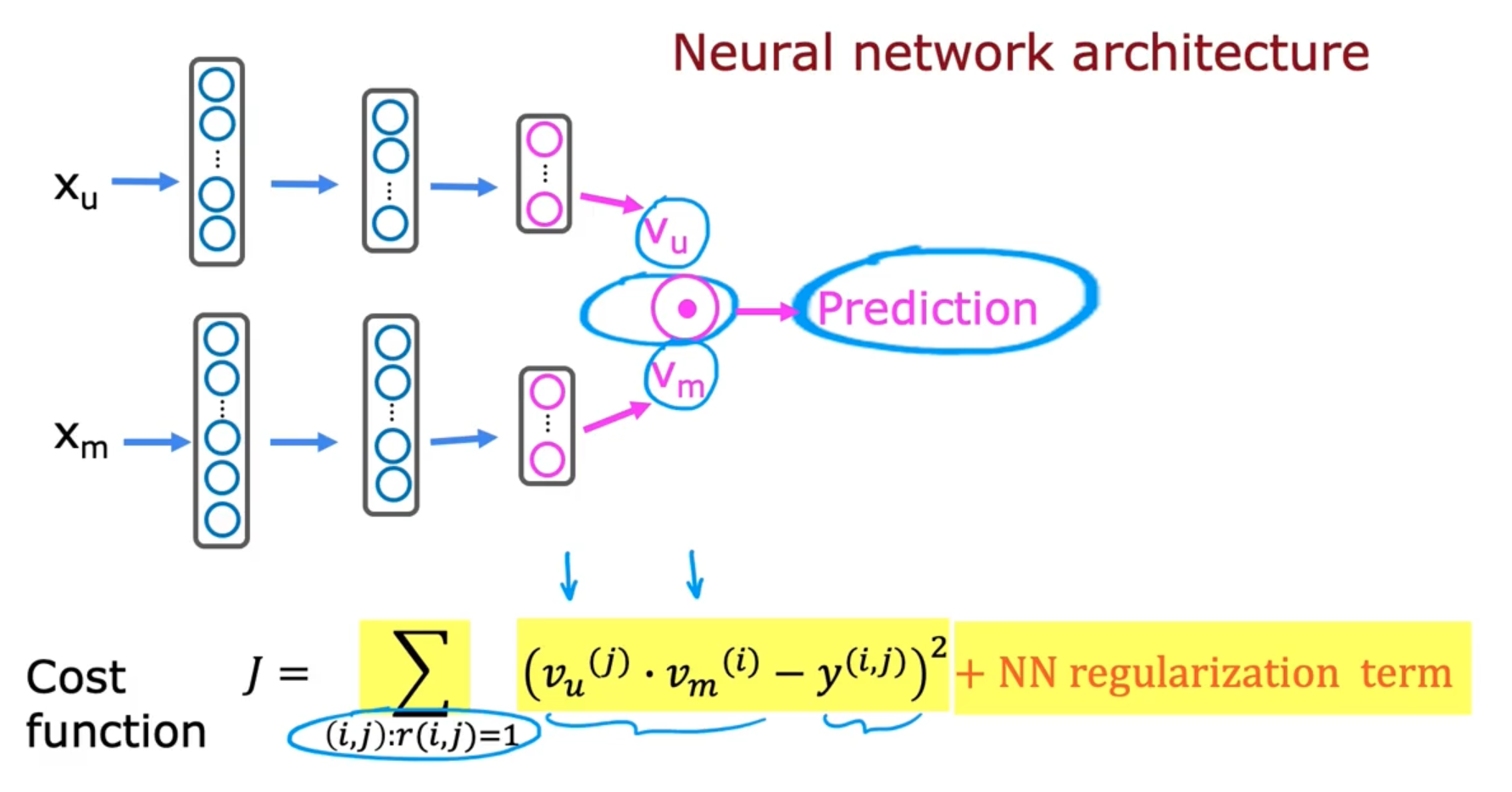
Learned user and item vectors:

$${\vec{v}}_u^{(j)}\text{ is a vector of length 32 that describes user }j\text{ with features }{\vec{x}}_u^{(j)}$$ $${\vec{v}}_m^{(i)}\text{ is a vector of length 32 that describes movie }i\text{ with features }{\vec{x}}_m^{(i)}$$ $$\text{To find movies similar to movie }i:$$ $${\Vert {\vec{v}}_m^{(k)}-{\vec{v}}_m^{(i)}\Vert }^2\text{small}$$ $${\Vert {\vec{x}}_m^{(k)}-{\vec{x}}_m^{(i)}\Vert }^2\text{small}$$ $$\text{Note: This can be pre-computed ahead of time}$$

Recommending from a large catelogue

How to efficiently find recommendation from a large set of items ? (It might be computationally inefficient to run neural network inference thousands of millions of times every time user shows up in a website )

Many large scale recommender systems are implemented in two steps as shown below: Retrieval :

• Generate large list of plausible item candidates (For example,)
  1. For each of the last 10 movies watched by the user, find 10 most similar movies
  2. For most viewed 3 genres, find the top 10 movies
  3. Top 20 movies in the country
• Combine retrieved items into list, removing duplicates and items already watched/purchased

Ranking :

1. Take list retrieved and rank using learned model
2. Display ranked items to user

• Retrieving more items results in a better performance, but slower recommendations. Based on our preference, we need to do find a trade-off point between the two

Principal Component Analysis

Used for visualization, specifically for dataset with a lot of features that cannot be plotted easily. PCA takes thousands of features, reduces it to two or three and then help to plot the features

PCA Algorithm

1. Find axis z(Principal component) to retain variance (info)
2. Find the projection points and use them as the new feature value

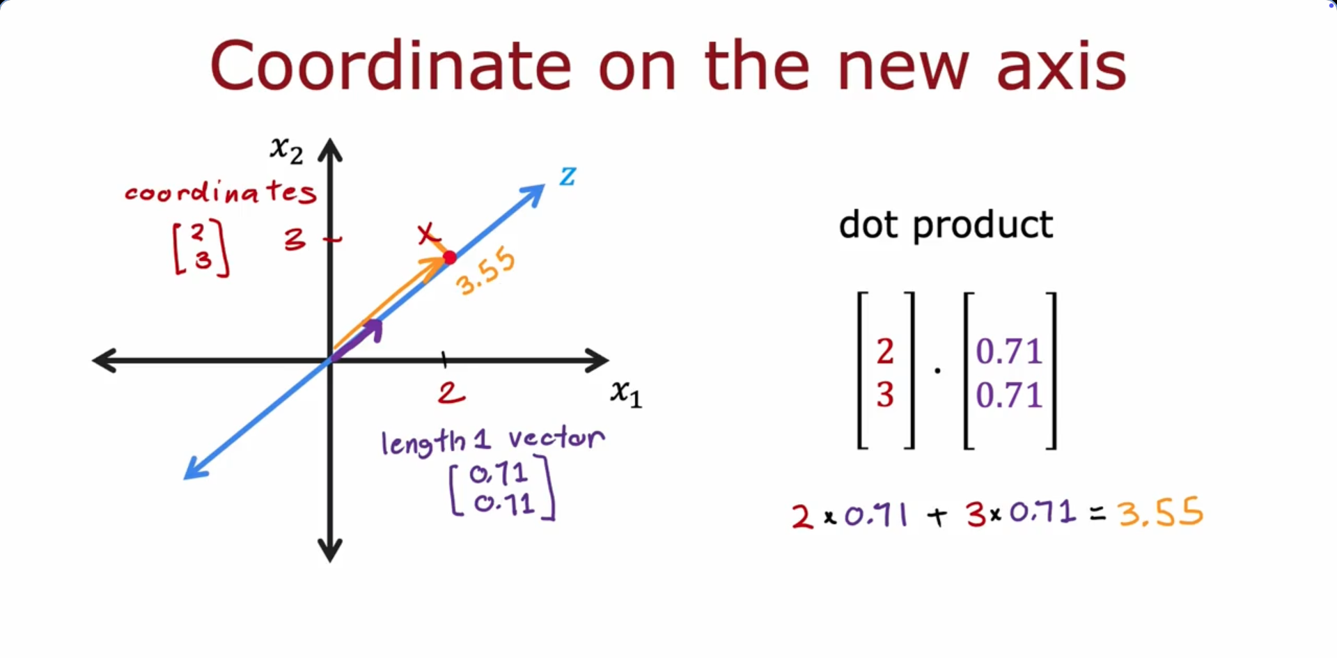
• Given a z value, we can use reconstruction to find the original (x${}_1$, x${}_2$)

Reinforcement Learning

What is Reinforcement Learning ?

A model learns to make decisions by interacting with an environment and receiving rewards or penalties for its actions

The Return in reinforcement learning

• The return is the sum of rewards that the system gets, weighted by the discount factor, where the rewards in a far future are weighted by a discount factor raised to a higher power
• If there are any rewards that are negative, then the discount factor will actually incentivize the system to push out the negative rewards as far into the future as possible (Applicable in financial applications)

Policy

In Reinforcement learning, our goal is to come up with a function which is called a policy (π) whose job is to take input state (S) and map it to action (a) that it wants us to take

• Find a policy π that tells you what action (a = π(s)) to take in every state (s) so as to maximize the return

Markov Decision Process (MDP) - Indicates that the future only depends on the current state and not on anything that might have occurred prior to of getting to current state

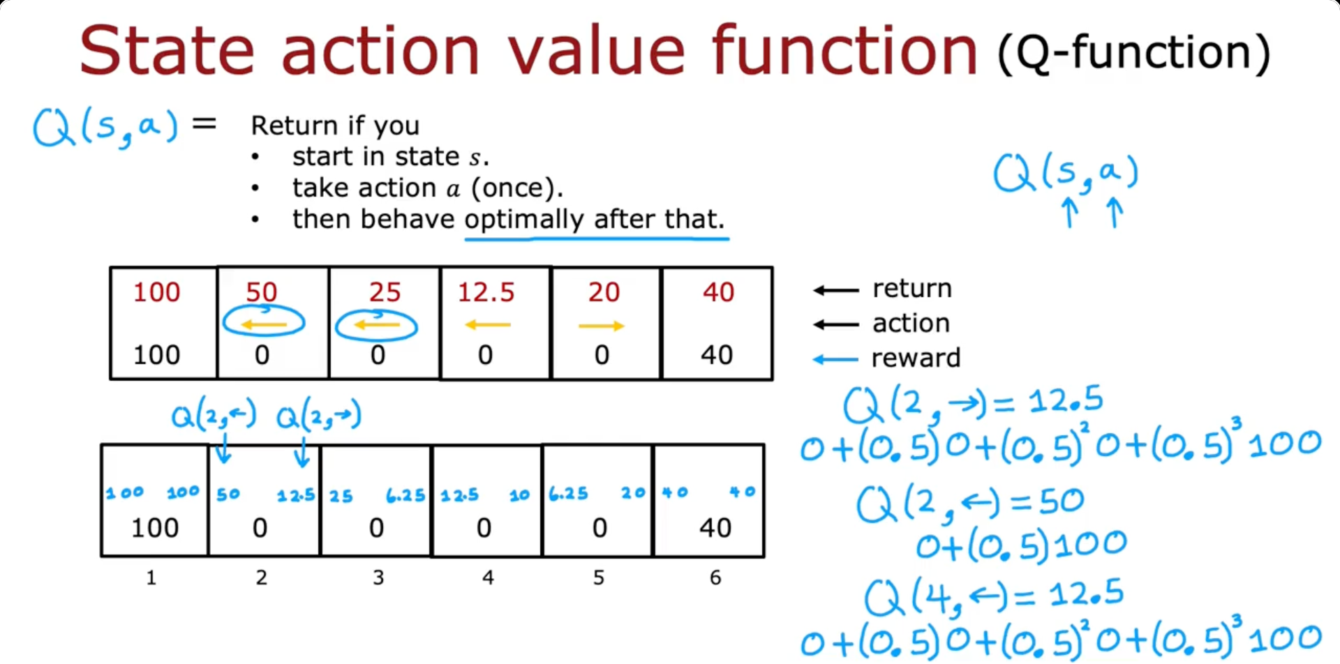
State-action value function

Q(s, a) = Return if we

• Start in state s.
• take action a (once)
• then behave optimally after that

The best possible return from state s is max Q(s, a) The best possible action in state s is the action a that gives max Q(s, a)

Bellman Equation

Helps us to calculate the state action value function Q(s, a)

Q(s, a) = Return if we

• Start in state s.
• take action a (once)
• then behave optimally after that

$$Q(s,a)=R(s)+\gamma \underset{a^{\prime }}{\max }Q(s^{\prime },a^{\prime })$$

$s$: current state $R(s)$ = reward of current state $a$: current action
$s^{\prime }$: state you get to after taking action $a$ $a^{\prime }$: action that you take in state $s^{\prime }$

Random (stochastic) environment

At times, in case of a stochastic environment, our Mars Rover may not exactly follow the action that we are asking it to take from a particular state. For example, it might slip and move right due to environmental factors though we command it to move left

• In such cases, we take the Expected Return (Average Return)

$$\text{Expected Return}=\text{Average}(R_1+\gamma R_2+{\gamma }^2{R}_3+{\gamma }^3{R}_4+\cdots )=\mathbb{E}\left[R_1+\gamma R_2+{\gamma }^2{R}_3+{\gamma }^3{R}_4+\cdots \right]$$ $$Q(s,a)=R(s)+\gamma E[\underset{a^{\prime }}{\max }Q(s^{\prime },a^{\prime })]$$

Continuous state spaces

• In case of a helicopter the following values are continuous. The state of a problem isn’t just one of a small number of possible discrete values (Ex: 1-6). Instead, it’s a vector of numbers any of which could take any values

1. Position x, y, z
2. Roll, Pitch, Yaw
3. Speed in x, y, z directions
4. Rate of turning (Angle of velocity) of Roll, Pitch, Yaw

Lunar Lander

Actions :

1. do nothing
2. left thruster (Moves to the right)
3. Main thruster (Located at the bottom)
4. right thruster (Moves to the left)

Reward Function :

1. Getting to landing pad: 100-140
2. Additional reward for moving toward/away from pad
3. Crash: -100
4. Soft Landing: +100
5. Leg grounded: +10
6. Fire main engine: -0.3
7. Fire side thruster: -0.03

Goal :

• Learn a policy $\pi$ that, given

$$s=\left[\begin{array}{c}x\\ y\\ \dot{x}\\ \dot{y}\\ \theta \\ \dot{\theta }\\ l\\ r\end{array}\right]$$

picks action $a=\pi (s)$ so as to maximize the return. ($\gamma =0.985$)

Learning the state-value function

DQN - Deep Q Network

1. Initialize neural network randomly as guess of $Q(s,a)$
2. Repeat{ Take actions in the lunar lander. Get $(s,a,R(s),s^{\prime })$ Store 10,000 most recent $(s,a,R(s),s^{\prime })$ tuples → Reply Buffer (Storing recent tuples) }
3. Train neural network: Create training set of 10,000 examples using $x=(s,a)$ and $y=R(s)+\gamma {\max }_{a^{\prime }}Q(s^{\prime },a^{\prime })$ Train $Q_{new}$ such that $Q_{new}(s,a)$ ~ y Set $Q=Q_{new}$

Algorithm Refinement

Improved neural network architecture

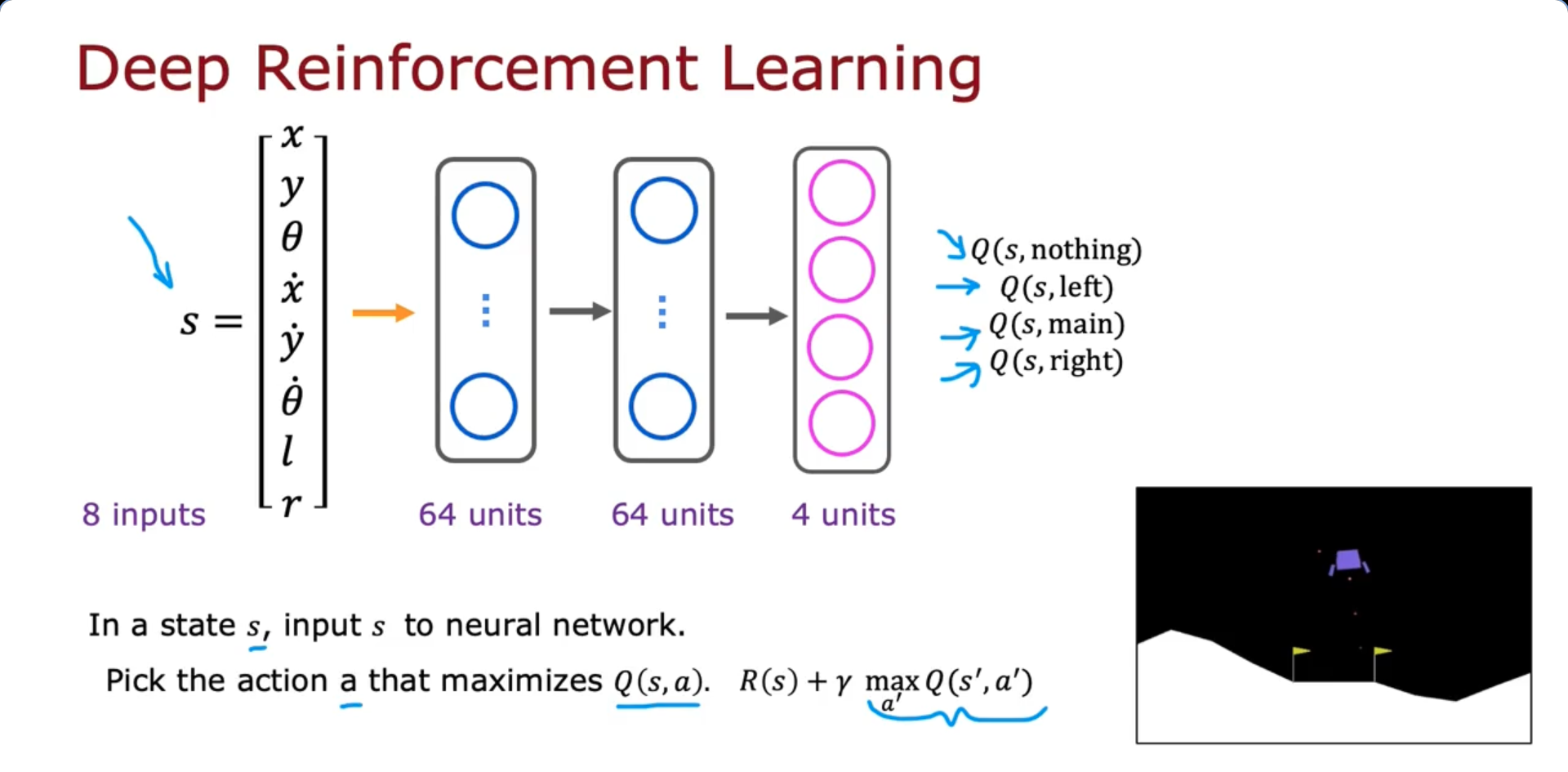
• In our previous architecture, with an input of 12 values, whenever we are in a state s, we would have to carry out inference separately four times to compute these four values $Q(s,nothing)$, $Q(s,left$, $Q(s,main)$, $Q(s,right)$ in order to pick the action that give the largest Q value. But, this is in-efficient because we have to carry out inference from every state four times
• It turns out to be more efficient to train a single neural network to output all four of the values simultaneously as shown in the above image

ε - greedy policy

How to choose action while still learning ?

In some state s Option 1: Pick the action a that maximizes $Q(s,a)$

Option 2:

• With probability 0.95, pick the action a that maximizes $Q(s,a)$ → Referred to as Greedy step or Exploitation step
• With Probability 0.05, pick an action $a$ randomly (Suppose the $Q(s,a)$ was initialized randomly so that the learning algorithm thinks firing the main thruster is never a good idea, the neural network parameters may be initialized such that $Q(s,main)$ is very low. If that’s the case, the neural network will never ever pick the action of firing the main thruster since it has a very low Q, thus it won’t ever learn that firing the main thruster is actually a good idea in case we follow only Option 1) → Referred to as Exploration step or ε - greedy policy (ε = 0.05)
• It’s common to start ε high and Gradually decrease so that eventually we are taking greedy actions mostly and random actions rarely

Mini-batch and soft update

Mini-batch

• In our Housing price prediction algorithm,

$$J(w,b)=\frac{1}{2m}\sum _{i=1}^m{\left(f_{w,b}(x^{(i)})-y^{(i)}\right)}^2$$ $$m=100,000,000$$ $$m^{\prime }=1,000$$

repeat {

$$w=w-\alpha \frac{\partial }{\partial w}\left(\frac{1}{2m^{\prime }}\sum _{i=1}^{m^{\prime }}{\left(f_{w,b}(x^{(i)})-y^{(i)}\right)}^2\right)$$ $$b=b-\alpha \frac{\partial }{\partial b}\left(\frac{1}{2m^{\prime }}\sum _{i=1}^{m^{\prime }}{\left(f_{w,b}(x^{(i)})-y^{(i)}\right)}^2\right)$$

}

• Taking the the Gradient-descent algorithm update step to consideration, in each step, we take summation of $m$ samples. When $m$ value is too large, the summation might be computationally expensive. So, instead of $m=100,000,000$, we take random $m^{\prime }=1,000$ entries from the sample during each updating step to enhance the algorithm

---

• Similarly, in our Reinforcement Learning Algorithm, we store $10,000$ most recent $(s,a,R(s),s^{\prime })$ tuples.
• While training the model, we create the training set of $1,000$ examples alone instead of $10,000$ examples which speeds up the entire process

Soft-update

• Abruptly updating the $Q$ value to $Q_{new}$ might affect the algorithm in case $Q_{new}$ turns out to be a bad value
• Making more gradual change to $Q$ or to update the original neural network parameters $w,B$ is a better choice

$$SetQ=Q_{new}$$ $$w=w_{new};b=b_{new}$$

Instead, update as follows :

$$w=0.01w_{new}+0.99w$$ $$B=0.01B_{new}+0.99B$$

The state of reinforcement learning

Limitations of Reinforcement Learning

• Much easier to get to work in a simulation than a real robot
• Far fewer applications than supervised and unsupervised learning
• But, exciting research direction with potential for future applications